Predictive Power Of Moving Averages

Table of Contents
Introduction #
The idea of time series momentum (AKA, trend following) heavily relies on the idea that if a price is higher than its recent moving average, it is more likely to continue to be higher than its moving average in the future, and vice versa. In this post, we will investigate the idea of moving averages, and whether at a given point in time a price that is higher or lower than the moving average up until that point in time has any predictive power for future returns.
Python Imports #
# Standard Library
import os
import sys
import warnings

from pathlib import Path

# Data Handling
import pandas as pd

# Suppress warnings
warnings.filterwarnings("ignore")
# Add the source subdirectory to the system path to allow import config from settings.py
current_directory = Path(os.getcwd())
website_base_directory = current_directory.parent.parent.parent
src_directory = website_base_directory / "src"
sys.path.append(str(src_directory)) if str(src_directory) not in sys.path else None

# Import settings.py
from settings import config

# Add configured directories from config to path
SOURCE_DIR = config("SOURCE_DIR")
sys.path.append(str(Path(SOURCE_DIR))) if str(Path(SOURCE_DIR)) not in sys.path else None

# Add other configured directories
BASE_DIR = config("BASE_DIR")
CONTENT_DIR = config("CONTENT_DIR")
POSTS_DIR = config("POSTS_DIR")
PAGES_DIR = config("PAGES_DIR")
PUBLIC_DIR = config("PUBLIC_DIR")
SOURCE_DIR = config("SOURCE_DIR")
DATA_DIR = config("DATA_DIR")
DATA_MANUAL_DIR = config("DATA_MANUAL_DIR")
Python Functions #
Here are the functions needed for this project:
- load_data: Load data from a CSV, Excel, or Pickle file into a pandas DataFrame.
- pandas_set_decimal_places: Set the number of decimal places displayed for floating-point numbers in pandas.
- plot_histogram: Plot the histogram of a data set from a DataFrame.
- plot_scatter: Plot the data from a DataFrame for a specified date range and columns.
- plot_time_series: Plot the timeseries data from a DataFrame for a specified date range and columns.
- run_regression: Run a linear regression using statsmodels OLS and return the results.
- summary_stats: Generate summary statistics for a series of returns.
- yf_pull_data: Download daily price data from Yahoo Finance and export it.
from load_data import load_data
from pandas_set_decimal_places import pandas_set_decimal_places
from plot_histogram import plot_histogram
from plot_scatter import plot_scatter
from plot_time_series import plot_time_series
from run_regression import run_regression
from summary_stats import summary_stats
from yf_pull_data import yf_pull_data
Data Overview #
For this exercise, we will investigate the predictive power of moving averages for the following ETFs:
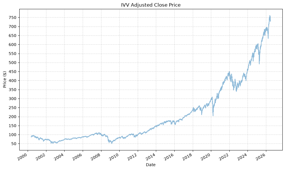
- IVV - iShares Core S&P 500 ETF
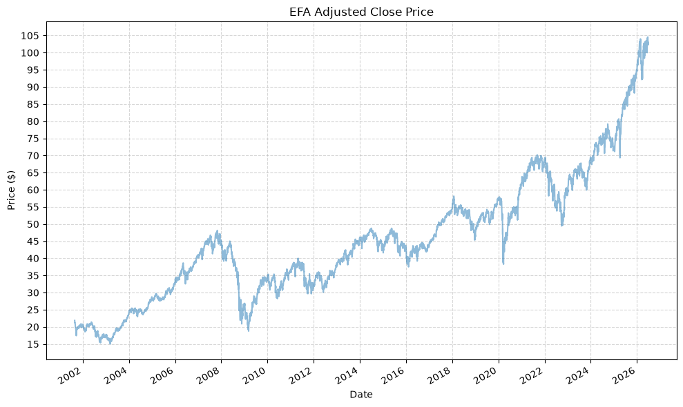
- EFA - iShares MSCI EAFE ETF
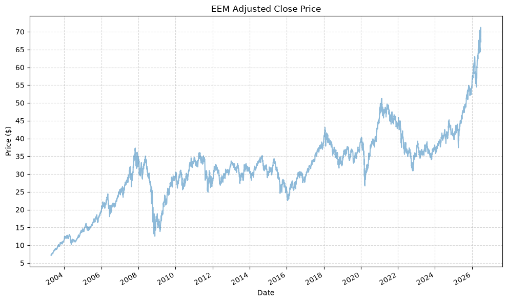
- EEM - iShares MSCI Emerging Markets ETF
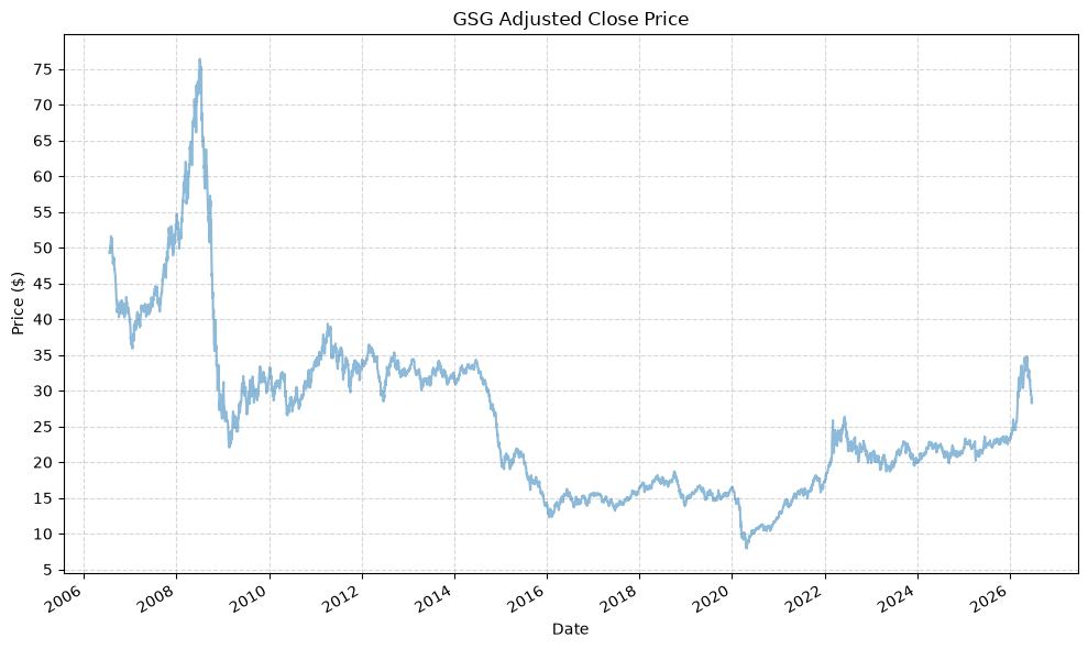
- GSG - iShares S&P GSCI Commodity-Indexed Trust
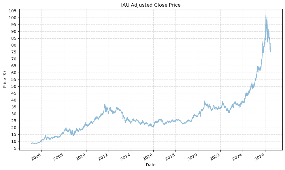
- IAU - iShares Gold Trust
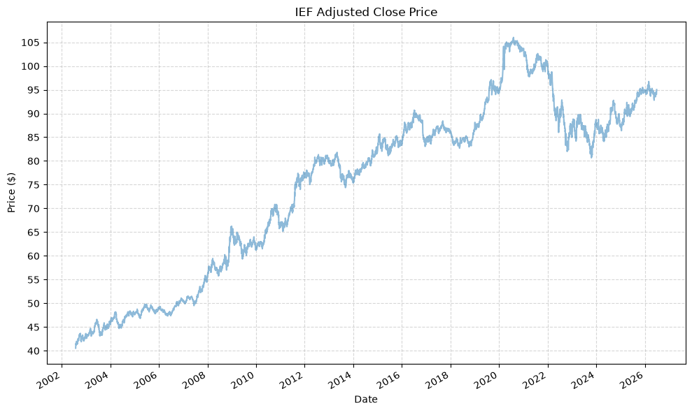
- IEF - iShares 7-10 Year Treasury Bond ETF
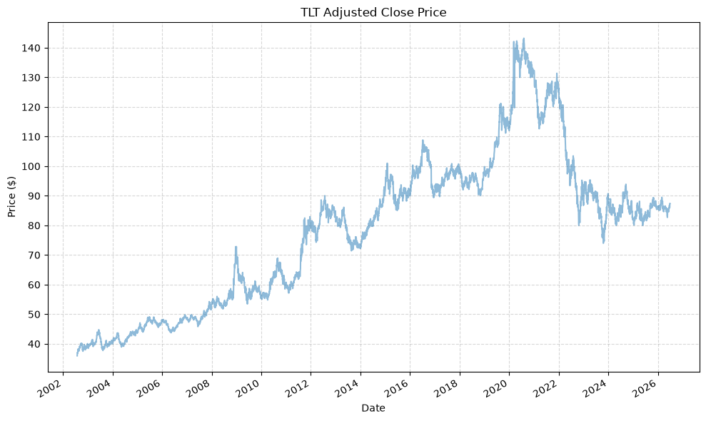
- TLT - iShares 20+ Year Treasury Bond ETF
We’ll use the adjusted close prices for each of these ETFs.
Acquire Data #
First, let’s get the data for these ETFs. If we already have the desired data, we can load it from a local pickle file. Otherwise, we can download it from Yahoo Finance using the yf_pull_data function.
pandas_set_decimal_places(2)

# Create a list of the ETF tickers
fund_list = ["IVV", "EFA", "EEM", "GSG", "IAU", "IEF", "TLT"]
# Pull data for each ETF and cache it locally
for fund in fund_list:
    yf_pull_data(
        base_directory=DATA_DIR,
        ticker=fund,
        adjusted=False,
        source="Yahoo_Finance",
        asset_class="Exchange_Traded_Funds",
        excel_export=True,
        pickle_export=True,
        output_confirmation=False,
    )
Create Data Dictionary #
Then, create a dictionary to hold the data for each ETF, and plot the adjusted close price for each ETF over time.
# Create an empty dictionary to hold the data for each ETF
fund_data = {}

# Load the data for each ETF, rename the columns to include the ticker, store it in the fund_data dictionary
for fund in fund_list:
    data = load_data(
        base_directory=DATA_DIR,
        ticker=fund,
        source="Yahoo_Finance",
        asset_class="Exchange_Traded_Funds",
        timeframe="Daily",
        file_format="pickle",
    )

    data = data.rename(columns={
        "Adj Close": f"{fund}_Adj_Close",
        "Close": f"{fund}_Close",
        "High": f"{fund}_High",
        "Low": f"{fund}_Low",
        "Open": f"{fund}_Open",
        "Volume": f"{fund}_Volume"
    })

    fund_data[fund] = data
Plot Data #
Next, we will:
- Check the date ranges
- Plot the adjusted close prices
- Plot the cumulative returns
- Plot the drawdowns
for fund, data in fund_data.items():
    display(data)

    plot_time_series(
        df=data,
        plot_start_date=None,
        plot_end_date=None,
        plot_columns=[f"{fund}_Adj_Close"],
        title=f"{fund} Adjusted Close Price",
        x_label="Date",
        x_format="Year",
        x_tick_spacing=2,
        x_tick_start=None,
        x_tick_rotation=30,
        y_label="Price ($)",
        y_format="Decimal",
        y_format_decimal_places=0,
        y_tick_spacing="Auto",
        y_tick_rotation=0,
        grid=True,
        legend=False,
        export_plot=False,
        plot_file_name=None,
    )
| IVV_Adj_Close | IVV_Close | IVV_High | IVV_Low | IVV_Open | IVV_Volume | |
|---|---|---|---|---|---|---|
| Date | ||||||
| 2000-05-19 | 88.33 | 140.69 | 142.66 | 140.25 | 142.66 | 775500 |
| 2000-05-22 | 87.79 | 139.81 | 140.59 | 136.81 | 140.59 | 1850600 |
| 2000-05-23 | 86.45 | 137.69 | 140.22 | 137.69 | 140.22 | 373900 |
| 2000-05-24 | 87.75 | 139.75 | 140.06 | 136.66 | 137.75 | 400300 |
| 2000-05-25 | 86.94 | 138.47 | 140.94 | 137.88 | 140.03 | 69600 |
| ... | ... | ... | ... | ... | ... | ... |
| 2026-06-22 | 747.78 | 747.78 | 753.66 | 746.58 | 751.16 | 16420300 |
| 2026-06-23 | 737.14 | 737.14 | 743.02 | 735.75 | 737.15 | 15553500 |
| 2026-06-24 | 736.66 | 736.66 | 743.40 | 734.26 | 738.56 | 9014700 |
| 2026-06-25 | 736.50 | 736.50 | 742.80 | 733.04 | 742.32 | 25573300 |
| 2026-06-26 | 730.17 | 730.17 | 739.97 | 728.74 | 732.29 | 5944000 |
6564 rows × 6 columns
| EFA_Adj_Close | EFA_Close | EFA_High | EFA_Low | EFA_Open | EFA_Volume | |
|---|---|---|---|---|---|---|
| Date | ||||||
| 2001-08-27 | 21.86 | 42.83 | 42.92 | 42.76 | 42.92 | 44700 |
| 2001-08-28 | 21.61 | 42.34 | 42.58 | 42.26 | 42.53 | 319800 |
| 2001-08-29 | 21.51 | 42.15 | 42.47 | 42.10 | 42.45 | 128400 |
| 2001-08-30 | 21.20 | 41.55 | 41.67 | 41.43 | 41.67 | 36900 |
| 2001-08-31 | 21.25 | 41.65 | 41.72 | 41.47 | 41.53 | 1656900 |
| ... | ... | ... | ... | ... | ... | ... |
| 2026-06-22 | 104.58 | 104.58 | 104.84 | 104.43 | 104.59 | 9596200 |
| 2026-06-23 | 102.46 | 102.46 | 103.02 | 102.32 | 102.38 | 17425700 |
| 2026-06-24 | 102.26 | 102.26 | 102.65 | 101.92 | 102.24 | 12504200 |
| 2026-06-25 | 103.15 | 103.15 | 103.73 | 102.73 | 103.48 | 13135400 |
| 2026-06-26 | 102.54 | 102.54 | 103.07 | 102.30 | 102.46 | 21219200 |
6244 rows × 6 columns
| EEM_Adj_Close | EEM_Close | EEM_High | EEM_Low | EEM_Open | EEM_Volume | |
|---|---|---|---|---|---|---|
| Date | ||||||
| 2003-04-14 | 7.20 | 11.22 | 11.22 | 11.14 | 11.14 | 93600 |
| 2003-04-15 | 7.28 | 11.36 | 11.39 | 11.29 | 11.29 | 421200 |
| 2003-04-16 | 7.37 | 11.49 | 11.53 | 11.48 | 11.48 | 9000 |
| 2003-04-17 | 7.42 | 11.57 | 11.57 | 11.53 | 11.55 | 17100 |
| 2003-04-21 | 7.42 | 11.56 | 11.58 | 11.56 | 11.58 | 72900 |
| ... | ... | ... | ... | ... | ... | ... |
| 2026-06-22 | 71.21 | 71.21 | 71.57 | 70.99 | 71.29 | 25302200 |
| 2026-06-23 | 67.17 | 67.17 | 68.23 | 67.07 | 67.25 | 39069000 |
| 2026-06-24 | 67.25 | 67.25 | 67.61 | 66.60 | 67.38 | 22973300 |
| 2026-06-25 | 67.96 | 67.96 | 68.99 | 67.27 | 68.91 | 24474400 |
| 2026-06-26 | 67.19 | 67.19 | 67.72 | 66.27 | 66.34 | 24158700 |
5838 rows × 6 columns
| GSG_Adj_Close | GSG_Close | GSG_High | GSG_Low | GSG_Open | GSG_Volume | |
|---|---|---|---|---|---|---|
| Date | ||||||
| 2006-07-21 | 49.25 | 49.25 | 49.64 | 49.22 | 49.35 | 37400 |
| 2006-07-24 | 49.70 | 49.70 | 49.70 | 48.98 | 49.25 | 220900 |
| 2006-07-25 | 49.25 | 49.25 | 50.15 | 49.20 | 50.15 | 41600 |
| 2006-07-26 | 49.62 | 49.62 | 49.80 | 49.35 | 49.35 | 17800 |
| 2006-07-27 | 50.15 | 50.15 | 50.35 | 49.93 | 50.15 | 41800 |
| ... | ... | ... | ... | ... | ... | ... |
| 2026-06-22 | 29.25 | 29.25 | 29.38 | 29.12 | 29.34 | 567600 |
| 2026-06-23 | 28.95 | 28.95 | 28.99 | 28.79 | 28.86 | 572000 |
| 2026-06-24 | 28.23 | 28.23 | 28.46 | 28.21 | 28.26 | 600700 |
| 2026-06-25 | 28.88 | 28.88 | 28.93 | 28.35 | 28.35 | 556900 |
| 2026-06-26 | 28.39 | 28.39 | 28.49 | 28.27 | 28.46 | 510000 |
5014 rows × 6 columns
| IAU_Adj_Close | IAU_Close | IAU_High | IAU_Low | IAU_Open | IAU_Volume | |
|---|---|---|---|---|---|---|
| Date | ||||||
| 2005-01-28 | 8.54 | 8.54 | 8.55 | 8.49 | 8.55 | 2888500 |
| 2005-01-31 | 8.45 | 8.45 | 8.46 | 8.40 | 8.45 | 759500 |
| 2005-02-01 | 8.42 | 8.42 | 8.43 | 8.39 | 8.42 | 347500 |
| 2005-02-02 | 8.45 | 8.45 | 8.45 | 8.41 | 8.45 | 1496500 |
| 2005-02-03 | 8.34 | 8.34 | 8.35 | 8.30 | 8.32 | 534000 |
| ... | ... | ... | ... | ... | ... | ... |
| 2026-06-22 | 78.80 | 78.80 | 79.18 | 78.42 | 78.75 | 9674400 |
| 2026-06-23 | 77.33 | 77.33 | 77.94 | 77.29 | 77.40 | 4652100 |
| 2026-06-24 | 74.99 | 74.99 | 76.01 | 74.44 | 74.78 | 10609200 |
| 2026-06-25 | 75.71 | 75.71 | 76.04 | 75.18 | 75.63 | 6287200 |
| 2026-06-26 | 76.56 | 76.56 | 77.02 | 76.07 | 76.29 | 4671800 |
5386 rows × 6 columns
| IEF_Adj_Close | IEF_Close | IEF_High | IEF_Low | IEF_Open | IEF_Volume | |
|---|---|---|---|---|---|---|
| Date | ||||||
| 2002-07-30 | 40.55 | 81.77 | 82.12 | 81.70 | 81.94 | 41300 |
| 2002-07-31 | 40.93 | 82.52 | 82.58 | 82.05 | 82.05 | 32600 |
| 2002-08-01 | 41.10 | 82.86 | 82.90 | 82.52 | 82.54 | 71400 |
| 2002-08-02 | 41.41 | 83.50 | 83.70 | 82.90 | 83.02 | 120300 |
| 2002-08-05 | 41.62 | 83.92 | 83.92 | 83.53 | 83.68 | 159300 |
| ... | ... | ... | ... | ... | ... | ... |
| 2026-06-22 | 94.00 | 94.00 | 94.13 | 93.97 | 94.11 | 4572200 |
| 2026-06-23 | 94.12 | 94.12 | 94.26 | 94.09 | 94.16 | 6504600 |
| 2026-06-24 | 94.73 | 94.73 | 94.78 | 94.56 | 94.57 | 5179800 |
| 2026-06-25 | 94.79 | 94.79 | 95.02 | 94.78 | 94.86 | 5630500 |
| 2026-06-26 | 95.03 | 95.03 | 95.08 | 94.83 | 94.83 | 5584100 |
6016 rows × 6 columns
| TLT_Adj_Close | TLT_Close | TLT_High | TLT_Low | TLT_Open | TLT_Volume | |
|---|---|---|---|---|---|---|
| Date | ||||||
| 2002-07-30 | 35.97 | 81.52 | 81.90 | 81.52 | 81.75 | 6100 |
| 2002-07-31 | 36.41 | 82.53 | 82.80 | 81.90 | 81.95 | 29400 |
| 2002-08-01 | 36.62 | 83.00 | 83.02 | 82.54 | 82.54 | 25000 |
| 2002-08-02 | 37.00 | 83.85 | 84.10 | 82.88 | 83.16 | 52800 |
| 2002-08-05 | 37.16 | 84.22 | 84.44 | 83.85 | 84.04 | 61100 |
| ... | ... | ... | ... | ... | ... | ... |
| 2026-06-22 | 86.09 | 86.09 | 86.33 | 85.97 | 86.30 | 28595100 |
| 2026-06-23 | 86.20 | 86.20 | 86.43 | 86.10 | 86.12 | 19145500 |
| 2026-06-24 | 87.38 | 87.38 | 87.47 | 87.12 | 87.15 | 41837000 |
| 2026-06-25 | 87.35 | 87.35 | 87.79 | 87.29 | 87.58 | 28380000 |
| 2026-06-26 | 87.36 | 87.36 | 87.37 | 87.00 | 87.01 | 21650800 |
6016 rows × 6 columns
# Create empty DF
data_merged = pd.DataFrame()

# Merge all data, calc cumulative returns, drawdowns
for fund, data in fund_data.items():
    data_merged = data_merged.merge(data[[f"{fund}_Adj_Close"]], left_index=True, right_index=True, how='outer') if not data_merged.empty else data[[f"{fund}_Adj_Close"]]
    data_merged[f"{fund}_Return"] = data_merged[f"{fund}_Adj_Close"].pct_change()
    data_merged[f"{fund}_Cumulative_Return"] = (1 + data_merged[f"{fund}_Return"]).cumprod() - 1
    data_merged[f"{fund}_Cumulative_Return_Plus_One"] = 1 + data_merged[f"{fund}_Cumulative_Return"]
    data_merged[f"{fund}_Rolling_Max"] = data_merged[f"{fund}_Cumulative_Return_Plus_One"].cummax()
    data_merged[f"{fund}_Drawdown"] = data_merged[f"{fund}_Cumulative_Return_Plus_One"] / data_merged[f"{fund}_Rolling_Max"] - 1
    data_merged.drop(columns=[f"{fund}_Cumulative_Return_Plus_One", f"{fund}_Rolling_Max"], inplace=True)

display(data_merged)
| IVV_Adj_Close | IVV_Return | IVV_Cumulative_Return | IVV_Drawdown | EFA_Adj_Close | EFA_Return | EFA_Cumulative_Return | EFA_Drawdown | EEM_Adj_Close | EEM_Return | ... | IAU_Cumulative_Return | IAU_Drawdown | IEF_Adj_Close | IEF_Return | IEF_Cumulative_Return | IEF_Drawdown | TLT_Adj_Close | TLT_Return | TLT_Cumulative_Return | TLT_Drawdown | |
|---|---|---|---|---|---|---|---|---|---|---|---|---|---|---|---|---|---|---|---|---|---|
| Date | |||||||||||||||||||||
| 2000-05-19 | 88.33 | NaN | NaN | NaN | NaN | NaN | NaN | NaN | NaN | NaN | ... | NaN | NaN | NaN | NaN | NaN | NaN | NaN | NaN | NaN | NaN |
| 2000-05-22 | 87.79 | -0.01 | -0.01 | 0.00 | NaN | NaN | NaN | NaN | NaN | NaN | ... | NaN | NaN | NaN | NaN | NaN | NaN | NaN | NaN | NaN | NaN |
| 2000-05-23 | 86.45 | -0.02 | -0.02 | -0.02 | NaN | NaN | NaN | NaN | NaN | NaN | ... | NaN | NaN | NaN | NaN | NaN | NaN | NaN | NaN | NaN | NaN |
| 2000-05-24 | 87.75 | 0.01 | -0.01 | -0.00 | NaN | NaN | NaN | NaN | NaN | NaN | ... | NaN | NaN | NaN | NaN | NaN | NaN | NaN | NaN | NaN | NaN |
| 2000-05-25 | 86.94 | -0.01 | -0.02 | -0.01 | NaN | NaN | NaN | NaN | NaN | NaN | ... | NaN | NaN | NaN | NaN | NaN | NaN | NaN | NaN | NaN | NaN |
| ... | ... | ... | ... | ... | ... | ... | ... | ... | ... | ... | ... | ... | ... | ... | ... | ... | ... | ... | ... | ... | ... |
| 2026-06-22 | 747.78 | -0.00 | 7.47 | -0.02 | 104.58 | 0.00 | 3.78 | 0.00 | 71.21 | 0.01 | ... | 8.23 | -0.22 | 94.00 | -0.00 | 1.32 | -0.11 | 86.09 | -0.01 | 1.39 | -0.40 |
| 2026-06-23 | 737.14 | -0.01 | 7.34 | -0.03 | 102.46 | -0.02 | 3.69 | -0.02 | 67.17 | -0.06 | ... | 8.06 | -0.24 | 94.12 | 0.00 | 1.32 | -0.11 | 86.20 | 0.00 | 1.40 | -0.40 |
| 2026-06-24 | 736.66 | -0.00 | 7.34 | -0.03 | 102.26 | -0.00 | 3.68 | -0.02 | 67.25 | 0.00 | ... | 7.78 | -0.26 | 94.73 | 0.01 | 1.34 | -0.11 | 87.38 | 0.01 | 1.43 | -0.39 |
| 2026-06-25 | 736.50 | -0.00 | 7.34 | -0.03 | 103.15 | 0.01 | 3.72 | -0.01 | 67.96 | 0.01 | ... | 7.87 | -0.25 | 94.79 | 0.00 | 1.34 | -0.11 | 87.35 | -0.00 | 1.43 | -0.39 |
| 2026-06-26 | 730.17 | -0.01 | 7.27 | -0.04 | 102.54 | -0.01 | 3.69 | -0.02 | 67.19 | -0.01 | ... | 7.97 | -0.25 | 95.03 | 0.00 | 1.34 | -0.10 | 87.36 | 0.00 | 1.43 | -0.39 |
6564 rows × 28 columns
And now the plots for the cumulative returns and drawdowns:
plot_time_series(
    df=data_merged,
    plot_start_date=None,
    plot_end_date=None,
    plot_columns=[col for col in data_merged.columns if "Cumulative_Return" in col],
    title="Cumulative Returns",
    x_label="Date",
    x_format="Year",
    x_tick_spacing=1,
    x_tick_start=None,
    x_tick_rotation=30,
    y_label="Cumulative Return",
    y_format="Decimal",
    y_format_decimal_places=0,
    y_tick_spacing="Auto",
    y_tick_rotation=0,
    grid=True,
    legend=True,
    export_plot=False,
    plot_file_name=None,
)

plot_time_series(
    df=data_merged,
    plot_start_date=None,
    plot_end_date=None,
    plot_columns=[col for col in data_merged.columns if "Drawdown" in col],
    title="Drawdowns",
    x_label="Date",
    x_format="Year",
    x_tick_spacing=1,
    x_tick_start=None,
    x_tick_rotation=30,
    y_label="Drawdown",
    y_format="Percentage",
    y_format_decimal_places=0,
    y_tick_spacing="Auto",
    y_tick_rotation=0,
    grid=True,
    legend=True,
    export_plot=False,
    plot_file_name=None,
)
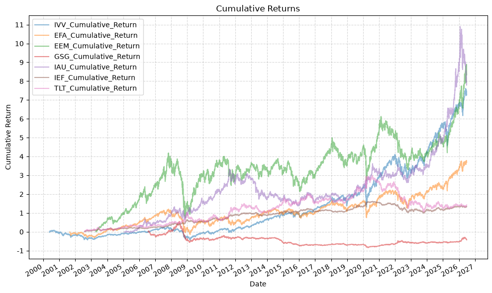
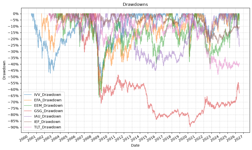
This time we’ll drop the empty rows to give a more accurate comparison, but this will reduce our data set to the inception of GSG in 2006:
# Create empty DF
data_merged_aligned = pd.DataFrame()

# Merge all data, calc cumulative returns, drawdowns
for fund, data in fund_data.items():
    data_merged_aligned = data_merged_aligned.merge(data[[f"{fund}_Adj_Close"]], left_index=True, right_index=True, how='outer') if not data_merged_aligned.empty else data[[f"{fund}_Adj_Close"]]
    data_merged_aligned = data_merged_aligned.dropna()

for fund in fund_data.keys():
    data_merged_aligned[f"{fund}_Return"] = data_merged_aligned[f"{fund}_Adj_Close"].pct_change()
    data_merged_aligned[f"{fund}_Cumulative_Return"] = (1 + data_merged_aligned[f"{fund}_Return"]).cumprod() - 1
    data_merged_aligned[f"{fund}_Cumulative_Return_Plus_One"] = 1 + data_merged_aligned[f"{fund}_Cumulative_Return"]
    data_merged_aligned[f"{fund}_Rolling_Max"] = data_merged_aligned[f"{fund}_Cumulative_Return_Plus_One"].cummax()
    data_merged_aligned[f"{fund}_Drawdown"] = data_merged_aligned[f"{fund}_Cumulative_Return_Plus_One"] / data_merged_aligned[f"{fund}_Rolling_Max"] - 1
    data_merged_aligned.drop(columns=[f"{fund}_Cumulative_Return_Plus_One", f"{fund}_Rolling_Max"], inplace=True)

display(data_merged_aligned)
| IVV_Adj_Close | EFA_Adj_Close | EEM_Adj_Close | GSG_Adj_Close | IAU_Adj_Close | IEF_Adj_Close | TLT_Adj_Close | IVV_Return | IVV_Cumulative_Return | IVV_Drawdown | ... | GSG_Drawdown | IAU_Return | IAU_Cumulative_Return | IAU_Drawdown | IEF_Return | IEF_Cumulative_Return | IEF_Drawdown | TLT_Return | TLT_Cumulative_Return | TLT_Drawdown | |
|---|---|---|---|---|---|---|---|---|---|---|---|---|---|---|---|---|---|---|---|---|---|
| Date | |||||||||||||||||||||
| 2006-07-21 | 85.98 | 34.42 | 19.76 | 49.25 | 12.37 | 48.32 | 45.51 | NaN | NaN | NaN | ... | NaN | NaN | NaN | NaN | NaN | NaN | NaN | NaN | NaN | NaN |
| 2006-07-24 | 87.44 | 35.04 | 20.65 | 49.70 | 12.22 | 48.32 | 45.49 | 0.02 | 0.02 | 0.00 | ... | 0.00 | -0.01 | -0.01 | 0.00 | 0.00 | 0.00 | 0.00 | -0.00 | -0.00 | 0.00 |
| 2006-07-25 | 87.78 | 35.03 | 20.70 | 49.25 | 12.34 | 48.28 | 45.35 | 0.00 | 0.02 | 0.00 | ... | -0.01 | 0.01 | -0.00 | 0.00 | -0.00 | -0.00 | -0.00 | -0.00 | -0.00 | -0.00 |
| 2006-07-26 | 87.95 | 35.28 | 20.62 | 49.62 | 12.40 | 48.40 | 45.52 | 0.00 | 0.02 | 0.00 | ... | -0.00 | 0.01 | 0.00 | 0.00 | 0.00 | 0.00 | 0.00 | 0.00 | 0.00 | 0.00 |
| 2006-07-27 | 87.83 | 35.50 | 20.90 | 50.15 | 12.59 | 48.39 | 45.45 | -0.00 | 0.02 | -0.00 | ... | 0.00 | 0.02 | 0.02 | 0.00 | -0.00 | 0.00 | -0.00 | -0.00 | -0.00 | -0.00 |
| ... | ... | ... | ... | ... | ... | ... | ... | ... | ... | ... | ... | ... | ... | ... | ... | ... | ... | ... | ... | ... | ... |
| 2026-06-22 | 747.78 | 104.58 | 71.21 | 29.25 | 78.80 | 94.00 | 86.09 | -0.00 | 7.70 | -0.02 | ... | -0.62 | -0.01 | 5.37 | -0.22 | -0.00 | 0.95 | -0.11 | -0.01 | 0.89 | -0.40 |
| 2026-06-23 | 737.14 | 102.46 | 67.17 | 28.95 | 77.33 | 94.12 | 86.20 | -0.01 | 7.57 | -0.03 | ... | -0.62 | -0.02 | 5.25 | -0.24 | 0.00 | 0.95 | -0.11 | 0.00 | 0.89 | -0.40 |
| 2026-06-24 | 736.66 | 102.26 | 67.25 | 28.23 | 74.99 | 94.73 | 87.38 | -0.00 | 7.57 | -0.03 | ... | -0.63 | -0.03 | 5.06 | -0.26 | 0.01 | 0.96 | -0.11 | 0.01 | 0.92 | -0.39 |
| 2026-06-25 | 736.50 | 103.15 | 67.96 | 28.88 | 75.71 | 94.79 | 87.35 | -0.00 | 7.57 | -0.03 | ... | -0.62 | 0.01 | 5.12 | -0.25 | 0.00 | 0.96 | -0.11 | -0.00 | 0.92 | -0.39 |
| 2026-06-26 | 730.17 | 102.54 | 67.19 | 28.39 | 76.56 | 95.03 | 87.36 | -0.01 | 7.49 | -0.04 | ... | -0.63 | 0.01 | 5.19 | -0.25 | 0.00 | 0.97 | -0.10 | 0.00 | 0.92 | -0.39 |
5014 rows × 28 columns
plot_time_series(
    df=data_merged_aligned,
    plot_start_date=None,
    plot_end_date=None,
    plot_columns=[col for col in data_merged_aligned.columns if "Cumulative_Return" in col],
    title="Cumulative Returns",
    x_label="Date",
    x_format="Year",
    x_tick_spacing=1,
    x_tick_start=None,
    x_tick_rotation=30,
    y_label="Cumulative Return",
    y_format="Decimal",
    y_format_decimal_places=1,
    y_tick_spacing="Auto",
    y_tick_rotation=0,
    grid=True,
    legend=True,
    export_plot=False,
    plot_file_name=None,
)

plot_time_series(
    df=data_merged_aligned,
    plot_start_date=None,
    plot_end_date=None,
    plot_columns=[col for col in data_merged_aligned.columns if "Drawdown" in col],
    title="Drawdowns",
    x_label="Date",
    x_format="Year",
    x_tick_spacing=1,
    x_tick_start=None,
    x_tick_rotation=30,
    y_label="Drawdown",
    y_format="Percentage",
    y_format_decimal_places=0,
    y_tick_spacing="Auto",
    y_tick_rotation=0,
    grid=True,
    legend=True,
    export_plot=False,
    plot_file_name=None,
)
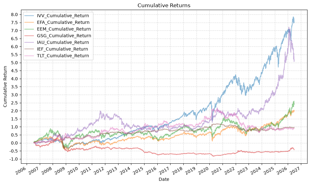
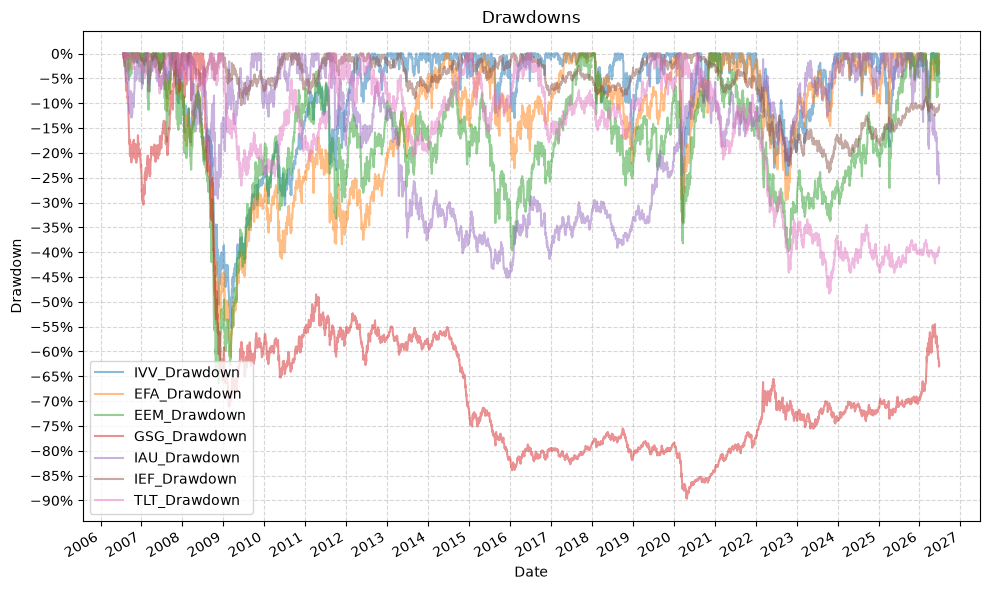
Several things to note here:
- Gold wins! Almost…
- You lose most of your money investing in commodies…
- Gold diversified well during the financial crisis
- The equity funds all had similar drawdowns
Summary Statistics #
Let’s look at the summary statistics. Keep in mind that we are not aligning the dates here, so the number of observations is different for each ETF.
sum_stats = pd.DataFrame()

for fund in fund_data.keys():
    data_stats = summary_stats(
        fund_list=[f"{fund}"],
        df=data_merged[[f"{fund}_Return"]].dropna(),
        period="Daily",
        use_calendar_days=False,
        excel_export=False,
        pickle_export=False,
        output_confirmation=False,
    )

    sum_stats = pd.concat([sum_stats, data_stats])

display(sum_stats)
| Number of Observations | Data Start Date | Data End Date | Annual Mean Return (Arithmetic) | Annualized Volatility | Annualized Sharpe Ratio | CAGR (Geometric) | Daily Max Return | Daily Max Return (Date) | Daily Min Return | Daily Min Return (Date) | Max Drawdown | Peak | Trough | Recovery Date | Calendar Days to Recovery | MAR Ratio | |
|---|---|---|---|---|---|---|---|---|---|---|---|---|---|---|---|---|---|
| IVV_Return | 6563 | 2000-05-22 | 2026-06-26 | 0.10 | 0.19 | 0.52 | 0.08 | 0.11 | 2008-10-28 | -0.12 | 2020-03-16 | -0.55 | 2007-10-09 | 2009-03-09 | 2012-08-16 | 1256.00 | 0.15 |
| EFA_Return | 6243 | 2001-08-28 | 2026-06-26 | 0.08 | 0.21 | 0.40 | 0.06 | 0.16 | 2008-10-13 | -0.11 | 2008-09-29 | -0.61 | 2007-10-31 | 2009-03-09 | 2014-06-06 | 1915.00 | 0.11 |
| EEM_Return | 5837 | 2003-04-15 | 2026-06-26 | 0.13 | 0.27 | 0.49 | 0.10 | 0.23 | 2008-10-13 | -0.16 | 2008-10-15 | -0.66 | 2007-10-31 | 2008-11-20 | 2017-09-18 | 3224.00 | 0.15 |
| GSG_Return | 5013 | 2006-07-24 | 2026-06-26 | -0.00 | 0.23 | -0.00 | -0.03 | 0.08 | 2008-11-04 | -0.12 | 2020-03-09 | -0.90 | 2008-07-02 | 2020-04-28 | NaT | NaN | -0.03 |
| IAU_Return | 5385 | 2005-01-31 | 2026-06-26 | 0.12 | 0.18 | 0.65 | 0.11 | 0.12 | 2008-09-17 | -0.10 | 2026-01-30 | -0.45 | 2011-08-22 | 2015-12-02 | 2020-07-27 | 1699.00 | 0.24 |
| IEF_Return | 6015 | 2002-07-31 | 2026-06-26 | 0.04 | 0.07 | 0.56 | 0.04 | 0.03 | 2009-03-18 | -0.03 | 2020-03-17 | -0.24 | 2020-08-04 | 2023-10-19 | NaT | NaN | 0.15 |
| TLT_Return | 6015 | 2002-07-31 | 2026-06-26 | 0.05 | 0.14 | 0.33 | 0.04 | 0.08 | 2020-03-20 | -0.07 | 2020-03-17 | -0.48 | 2020-08-04 | 2023-10-19 | NaT | NaN | 0.08 |
Calculate Moving Averages #
Now, let’s calculate the various different moving averages for each ETF. We will calculate the 3, 4, 5, 6, 7, 8, 9, 10, 11, and 12 month moving averages, using the equivalent number of trading days for each time period (63, 84, 105, 126, 147, 168, 189, 210, 231, and 252 trading days).
# Define moving average windows in trading days
ma_windows = {
    '3m': 63,     # 3 months (~63 trading days)
    '4m': 84,     # 4 months (~84 trading days)
    '5m': 105,    # 5 months (~105 trading days)
    '6m': 126,    # 6 months (~126 trading days)
    '7m': 147,    # 7 months (~147 trading days)
    '8m': 168,    # 8 months (~168 trading days)
    '9m': 189,    # 9 months (~189 trading days)
    '10m': 210,   # 10 months (~210 trading days)
    '11m': 231,   # 11 months (~231 trading days)
    '12m': 252    # 12 months (~252 trading days)
}
for fund, data in fund_data.items():
    for window, days in ma_windows.items():
        data[f"{fund}_MA_{window}"] = data[f"{fund}_Adj_Close"].rolling(window=days).mean()
Calculate Forward Return Windows #
Next, we will calculate the forward return for each ETF for the same time periods as the moving averages. For example, we will calculate the 3 month forward return, which is the return from the current date to 3 months in the future, and so on for each of the other time periods.
# Define forward return windows in trading days
forward_return_windows = {
    '3m': 63,     # 3 months (~63 trading days)
    '4m': 84,     # 4 months (~84 trading days)
    '5m': 105,    # 5 months (~105 trading days)
    '6m': 126,    # 6 months (~126 trading days)
    '7m': 147,    # 7 months (~147 trading days)
    '8m': 168,    # 8 months (~168 trading days)
    '9m': 189,    # 9 months (~189 trading days)
    '10m': 210,   # 10 months (~210 trading days)
    '11m': 231,   # 11 months (~231 trading days)
    '12m': 252    # 12 months (~252 trading days)
}
for fund, data in fund_data.items():
    for window, days in forward_return_windows.items():
        data[f"{fund}_Forward_Return_{window}"] = data[f"{fund}_Adj_Close"].shift(-days) / data[f"{fund}_Adj_Close"] - 1
Calculate Moving Average Predictions #
Now, we will calculate the moving average predictions, as follows:
- If the price is above the moving average, the prediction is 1 (i.e. the price will be above the moving average in the future).
- If the price is below the moving average, the prediction is -1 (i.e. the price will be below the moving average in the future).
- Calculate the accuracy of the predictions by comparing them to the actual forward returns (i.e. if the forward return is positive, the actual outcome is 1, and if the forward return is negative, the actual outcome is -1).
- Calculate the difference between the price and moving average (percentage), z-score (standardize) both that difference and the forward returns, and run a standardized OLS regression of forward return on the price-MA difference. Standardizing both sides puts every fund, moving average, and forward return window on the same scale, so the regression slope (a standardized beta, equal to the Pearson correlation) is directly comparable across them.
ma_prediction_results = pd.DataFrame(columns=[
    "Fund",
    "MA_Window",
    "Forward_Return_Window",
    "Overall_Accuracy",
    "Positive_Accuracy",
    "Negative_Accuracy",
    "Std_Beta",
    "Std_Beta_PValue",
    "R_Squared",
])

for fund, data in fund_data.items():
    for ma_label, ma_window in ma_windows.items():
        # Prediction and the price-vs-MA gap depend only on the MA window, so compute them
        # once per MA on the full frame (these columns persist for the plots further down).
        data[f"{fund}_MA_Prediction_{ma_label}"] = 0
        data.loc[data[f"{fund}_Adj_Close"] > data[f"{fund}_MA_{ma_label}"], f"{fund}_MA_Prediction_{ma_label}"] = 1
        data.loc[data[f"{fund}_Adj_Close"] < data[f"{fund}_MA_{ma_label}"], f"{fund}_MA_Prediction_{ma_label}"] = -1

        # Calculate the percentage difference between price and moving average
        data[f"{fund}_Price_MA_Diff_Percent_{ma_label}"] = (data[f"{fund}_Adj_Close"] - data[f"{fund}_MA_{ma_label}"]) / data[f"{fund}_MA_{ma_label}"]

        for fr_label, fr_window in forward_return_windows.items():
            data[f"{fund}_Actual_{fr_label}"] = 0
            data.loc[data[f"{fund}_Forward_Return_{fr_label}"] > 0, f"{fund}_Actual_{fr_label}"] = 1
            data.loc[data[f"{fund}_Forward_Return_{fr_label}"] < 0, f"{fund}_Actual_{fr_label}"] = -1

            pred_col = f"{fund}_MA_Prediction_{ma_label}"
            actual_col = f"{fund}_Actual_{fr_label}"
            diff_col = f"{fund}_Price_MA_Diff_Percent_{ma_label}"
            fr_col = f"{fund}_Forward_Return_{fr_label}"

            # Restrict to rows where THIS MA and THIS forward return are both defined, so each
            # window pair is evaluated on its own full sample rather than the intersection of all
            # 12 windows. (Dropping NaN on every column collapsed every pair onto the 12m-MA /
            # 12m-forward overlap, discarding most of the data for the shorter windows.)
            pair_data = data.dropna(subset=[f"{fund}_MA_{ma_label}", fr_col])
            # pair_data = pair_data.resample("W").last()

            overall_accuracy = (pair_data[pred_col] == pair_data[actual_col]).mean()
            pos_accuracy = ((pair_data[pred_col] == 1) & (pair_data[actual_col] == 1)).sum() / (pair_data[pred_col] == 1).sum()
            neg_accuracy = ((pair_data[pred_col] == -1) & (pair_data[actual_col] == -1)).sum() / (pair_data[pred_col] == -1).sum()

            # Calculate the mean forward return (and +/- 2 std bands) for the cases where the MA predicted a positive return and where it predicted a negative return
            positive_returns = pair_data.loc[pair_data[pred_col] == 1, fr_col]
            positive_mean_return = positive_returns.mean()
            positive_mean_plus_two_std = positive_mean_return + positive_returns.std() * 2
            positive_mean_minus_two_std = positive_mean_return - positive_returns.std() * 2
            negative_returns = pair_data.loc[pair_data[pred_col] == -1, fr_col]
            negative_mean_return = negative_returns.mean()
            negative_mean_plus_two_std = negative_mean_return + negative_returns.std() * 2
            negative_mean_minus_two_std = negative_mean_return - negative_returns.std() * 2

            # Z-score (standardize) the predictor and the forward return so the regression
            # slope is a standardized beta, comparable across funds, MAs, and forward windows.
            # With both sides standardized the slope equals the Pearson correlation.
            diff_z_col = f"{diff_col}_Z"
            fr_z_col = f"{fr_col}_Z"
            pair_data = pair_data.assign(**{
                diff_z_col: (pair_data[diff_col] - pair_data[diff_col].mean()) / pair_data[diff_col].std(),
                fr_z_col: (pair_data[fr_col] - pair_data[fr_col].mean()) / pair_data[fr_col].std(),
            })

            # Run a standardized OLS regression of forward return on the price-MA difference
            model = run_regression(
                df=pair_data,
                x_plot_column=diff_z_col,
                y_plot_column=fr_z_col,
                regression_model="OLS-statsmodels",
                regression_constant=True,
            )
            std_beta = model.params.iloc[1]          # standardized slope (== Pearson correlation)
            std_beta_pvalue = model.pvalues.iloc[1]  # p-value for the slope
            r_squared = model.rsquared               # R-squared of the regression

            results = pd.DataFrame([{
                    "Fund": fund,
                    "MA_Window": ma_label,
                    "Forward_Return_Window": fr_label,
                    "Overall_Accuracy": overall_accuracy,
                    "Positive_Accuracy": pos_accuracy,
                    "Negative_Accuracy": neg_accuracy,
                    "Positive_Mean_Return": positive_mean_return,
                    "Positive_Mean_Plus_Two_Std": positive_mean_plus_two_std,
                    "Positive_Mean_Minus_Two_Std": positive_mean_minus_two_std,
                    "Negative_Mean_Return": negative_mean_return,
                    "Negative_Mean_Plus_Two_Std": negative_mean_plus_two_std,
                    "Negative_Mean_Minus_Two_Std": negative_mean_minus_two_std,
                    "Std_Beta": std_beta,
                    "Std_Beta_PValue": std_beta_pvalue,
                    "R_Squared": r_squared,
            }])

            ma_prediction_results = pd.concat([ma_prediction_results, results], ignore_index=True)
display(ma_prediction_results)
| Fund | MA_Window | Forward_Return_Window | Overall_Accuracy | Positive_Accuracy | Negative_Accuracy | Std_Beta | Std_Beta_PValue | R_Squared | Positive_Mean_Return | Positive_Mean_Plus_Two_Std | Positive_Mean_Minus_Two_Std | Negative_Mean_Return | Negative_Mean_Plus_Two_Std | Negative_Mean_Minus_Two_Std | |
|---|---|---|---|---|---|---|---|---|---|---|---|---|---|---|---|
| 0 | IVV | 3m | 3m | 0.59 | 0.71 | 0.34 | -0.01 | 0.30 | 0.00 | 0.02 | 0.15 | -0.10 | 0.02 | 0.23 | -0.18 |
| 1 | IVV | 3m | 4m | 0.61 | 0.73 | 0.35 | 0.02 | 0.05 | 0.00 | 0.03 | 0.18 | -0.11 | 0.03 | 0.26 | -0.21 |
| 2 | IVV | 3m | 5m | 0.64 | 0.76 | 0.36 | 0.03 | 0.02 | 0.00 | 0.04 | 0.21 | -0.12 | 0.03 | 0.30 | -0.24 |
| 3 | IVV | 3m | 6m | 0.64 | 0.77 | 0.35 | 0.02 | 0.10 | 0.00 | 0.05 | 0.24 | -0.14 | 0.04 | 0.33 | -0.25 |
| 4 | IVV | 3m | 7m | 0.66 | 0.80 | 0.36 | 0.04 | 0.00 | 0.00 | 0.06 | 0.27 | -0.14 | 0.05 | 0.36 | -0.27 |
| ... | ... | ... | ... | ... | ... | ... | ... | ... | ... | ... | ... | ... | ... | ... | ... |
| 695 | TLT | 12m | 8m | 0.46 | 0.54 | 0.34 | -0.07 | 0.00 | 0.01 | 0.02 | 0.23 | -0.19 | 0.04 | 0.26 | -0.18 |
| 696 | TLT | 12m | 9m | 0.46 | 0.56 | 0.31 | -0.06 | 0.00 | 0.00 | 0.03 | 0.25 | -0.20 | 0.04 | 0.27 | -0.19 |
| 697 | TLT | 12m | 10m | 0.47 | 0.58 | 0.31 | -0.06 | 0.00 | 0.00 | 0.03 | 0.27 | -0.21 | 0.04 | 0.29 | -0.20 |
| 698 | TLT | 12m | 11m | 0.49 | 0.61 | 0.32 | -0.04 | 0.01 | 0.00 | 0.04 | 0.28 | -0.21 | 0.05 | 0.30 | -0.21 |
| 699 | TLT | 12m | 12m | 0.50 | 0.63 | 0.33 | -0.02 | 0.13 | 0.00 | 0.04 | 0.30 | -0.22 | 0.05 | 0.31 | -0.22 |
700 rows × 15 columns
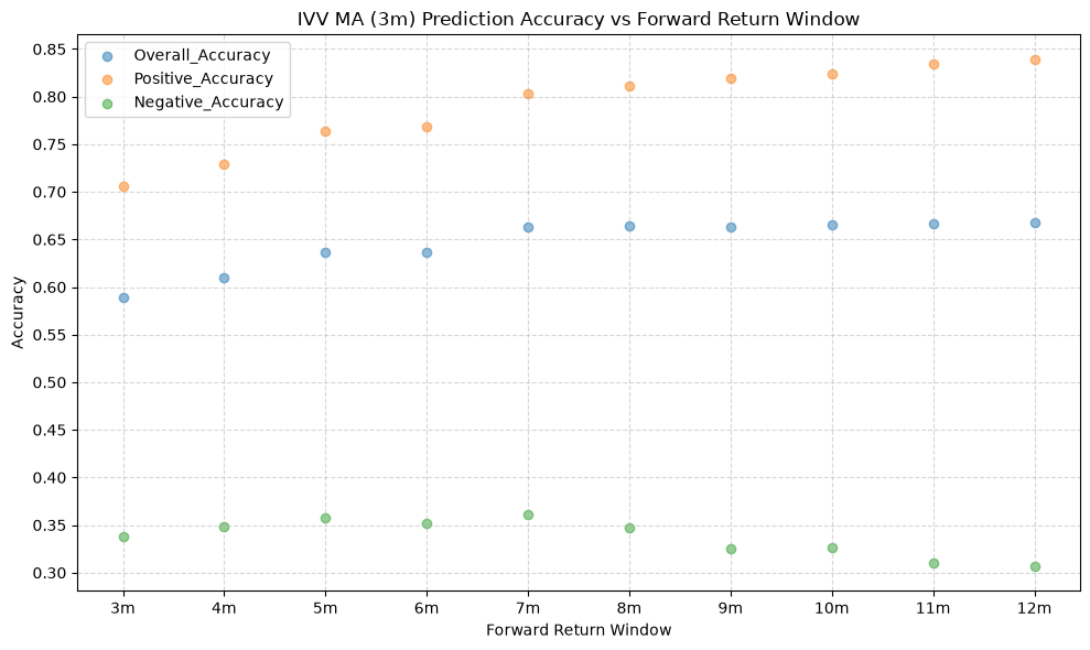
Plot Moving Average Predictions #
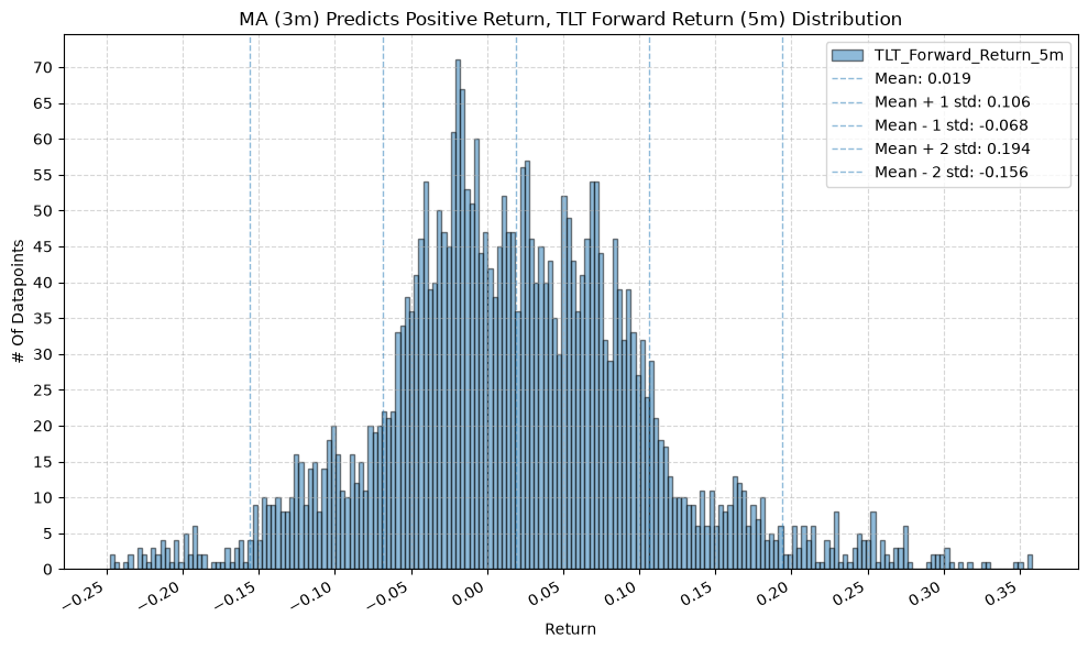
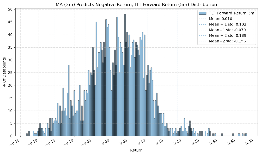
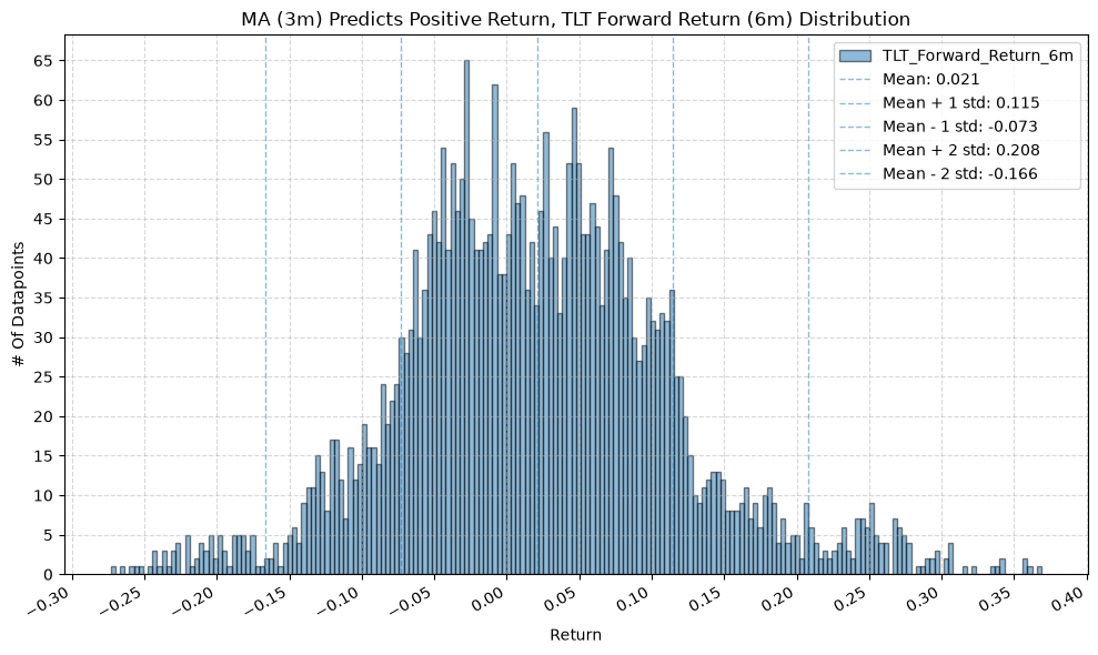
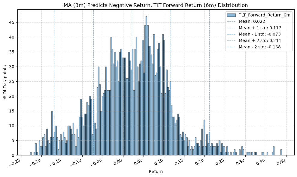
The following plots show the relationship between the price-MA difference and the forward returns for each ETF, moving average, and forward return window. Simply comment out the MA and forward return windows you don’t want to plot. we’ll use the 3 month MA for a brief look at the results.
# Define moving average windows in trading days
ma_windows = {
    '3m': 63,     # 3 months (~63 trading days)
    # '4m': 84,     # 4 months (~84 trading days)
    # '5m': 105,    # 5 months (~105 trading days)
    # '6m': 126,    # 6 months (~126 trading days)
    # '7m': 147,    # 7 months (~147 trading days)
    # '8m': 168,    # 8 months (~168 trading days)
    # '9m': 189,    # 9 months (~189 trading days)
    # '10m': 210,   # 10 months (~210 trading days)
    # '11m': 231,   # 11 months (~231 trading days)
    # '12m': 252    # 12 months (~252 trading days)
}

# Define forward return windows in trading days
forward_return_windows = {
    '3m': 63,     # 3 months (~63 trading days)
    '4m': 84,     # 4 months (~84 trading days)
    '5m': 105,    # 5 months (~105 trading days)
    '6m': 126,    # 6 months (~126 trading days)
    '7m': 147,    # 7 months (~147 trading days)
    '8m': 168,    # 8 months (~168 trading days)
    '9m': 189,    # 9 months (~189 trading days)
    '10m': 210,   # 10 months (~210 trading days)
    '11m': 231,   # 11 months (~231 trading days)
    '12m': 252    # 12 months (~252 trading days)
}
IVV, EFA, and EEM #
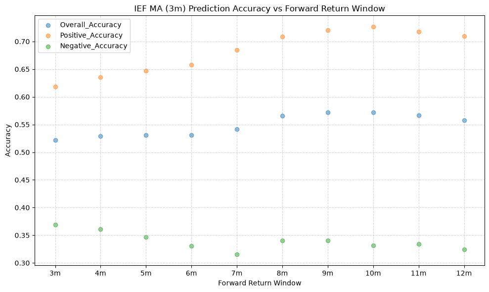
for fund, data in fund_data.items():
if fund not in ["IVV", "EFA", "EEM"]:
continue
for ma_label, ma_window in ma_windows.items():
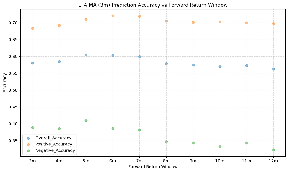
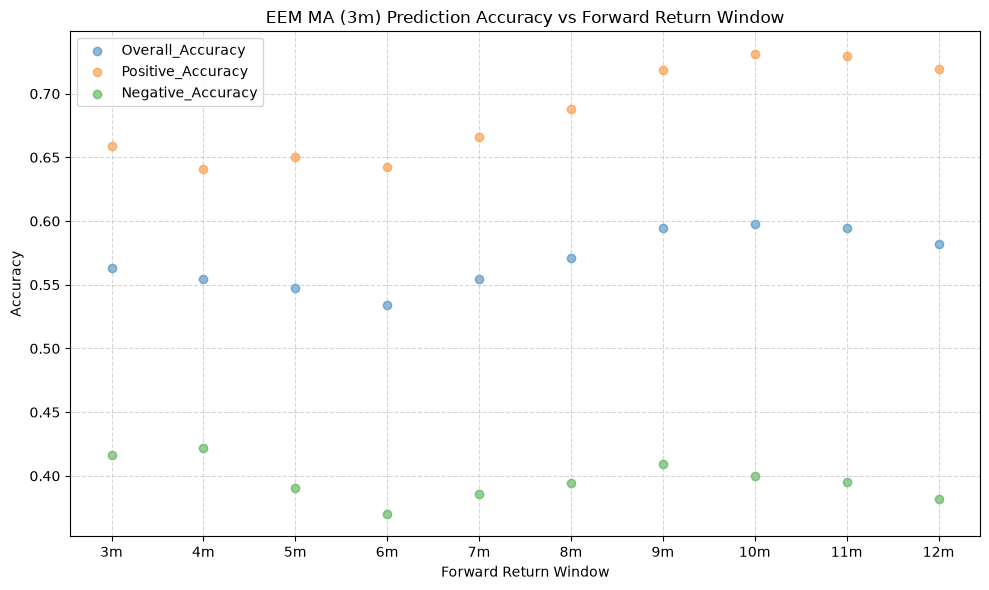
plot_scatter(
df=ma_prediction_results[(ma_prediction_results["Fund"] == fund) & (ma_prediction_results["MA_Window"] == ma_label)],
x_plot_column="Forward_Return_Window",
y_plot_columns=["Overall_Accuracy", "Positive_Accuracy", "Negative_Accuracy"],
title=f"{fund} MA ({ma_label}) Prediction Accuracy vs Forward Return Window",
x_label="Forward Return Window",
x_format="String",
x_format_decimal_places=0,
x_tick_spacing=1,
x_tick_start=None,
x_tick_rotation=0,
y_label="Accuracy",
y_format="Decimal",
y_format_decimal_places=2,
y_tick_spacing="Auto",
y_tick_rotation=0,
plot_OLS_regression_line=False,
OLS_column=None,
plot_Ridge_regression_line=False,
Ridge_column=None,
plot_RidgeCV_regression_line=False,
RidgeCV_column=None,
regression_constant=True,
grid=True,
legend=True,
export_plot=False,
plot_file_name=None,
)
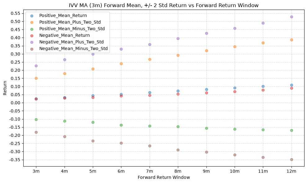
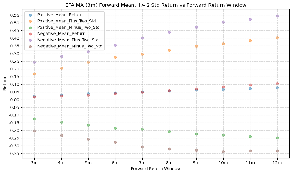
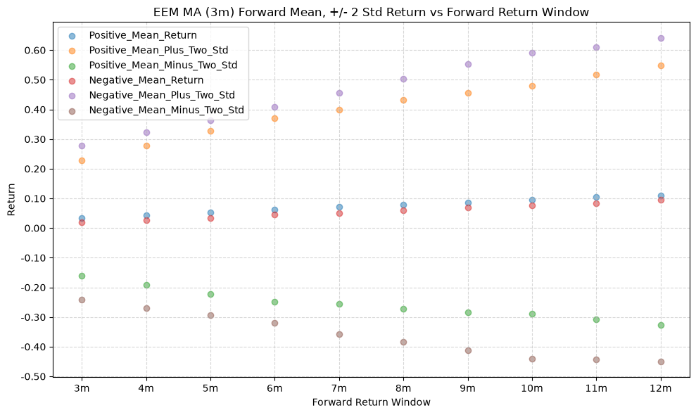
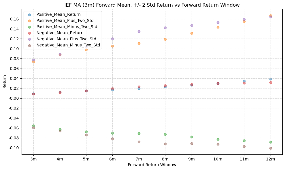
plot_scatter(
df=ma_prediction_results[(ma_prediction_results["Fund"] == fund) & (ma_prediction_results["MA_Window"] == ma_label)],
x_plot_column="Forward_Return_Window",
y_plot_columns=["Positive_Mean_Return", "Positive_Mean_Plus_Two_Std", "Positive_Mean_Minus_Two_Std", "Negative_Mean_Return", "Negative_Mean_Plus_Two_Std", "Negative_Mean_Minus_Two_Std"],
title=f"{fund} MA ({ma_label}) Forward Mean, +/- 2 Std Return vs Forward Return Window",
x_label="Forward Return Window",
x_format="String",
x_format_decimal_places=0,
x_tick_spacing=1,
x_tick_start=None,
x_tick_rotation=0,
y_label="Return",
y_format="Decimal",
y_format_decimal_places=2,
y_tick_spacing="Auto",
y_tick_rotation=0,
plot_OLS_regression_line=False,
OLS_column=None,
plot_Ridge_regression_line=False,
Ridge_column=None,
plot_RidgeCV_regression_line=False,
RidgeCV_column=None,
regression_constant=True,
grid=True,
legend=True,
export_plot=False,
plot_file_name=None,
)
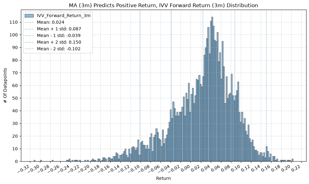
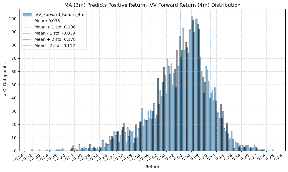
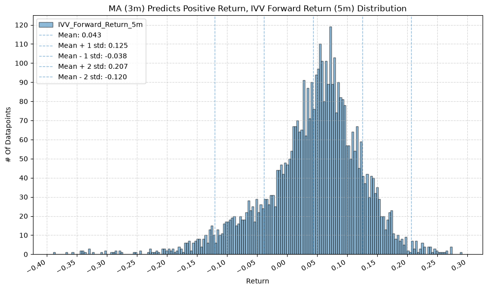
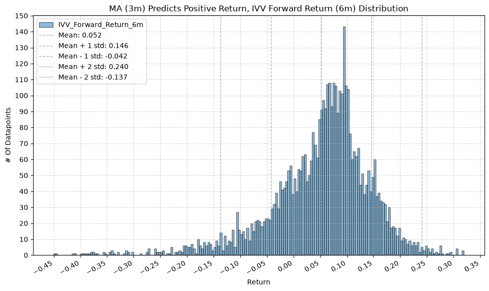
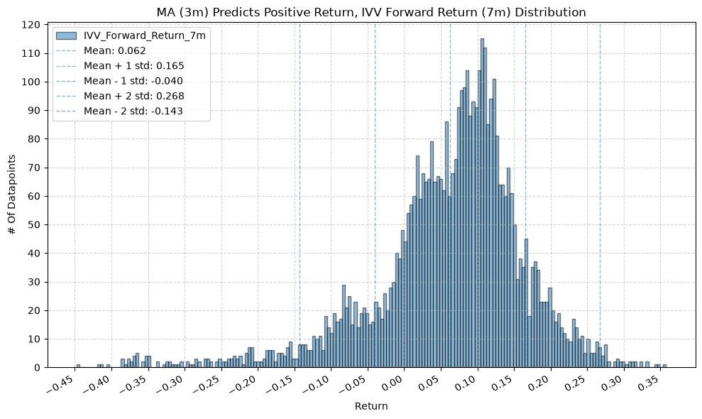
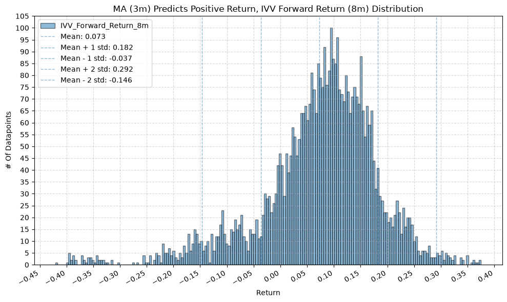
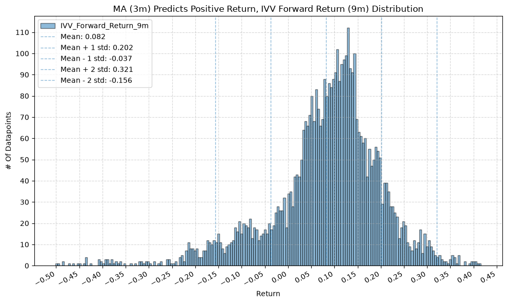
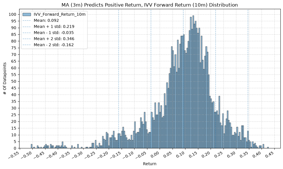
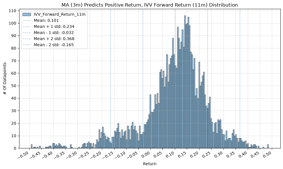
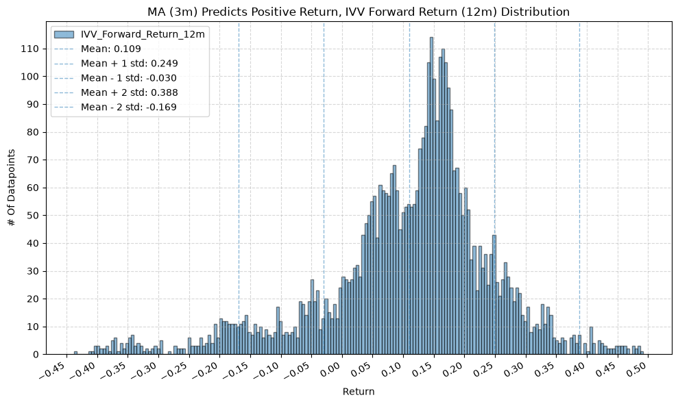
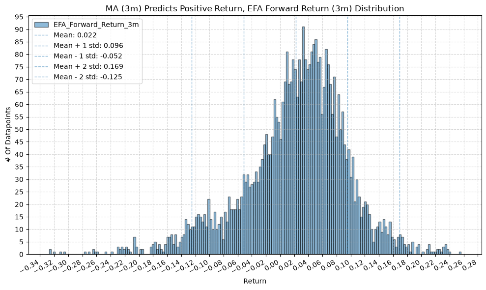
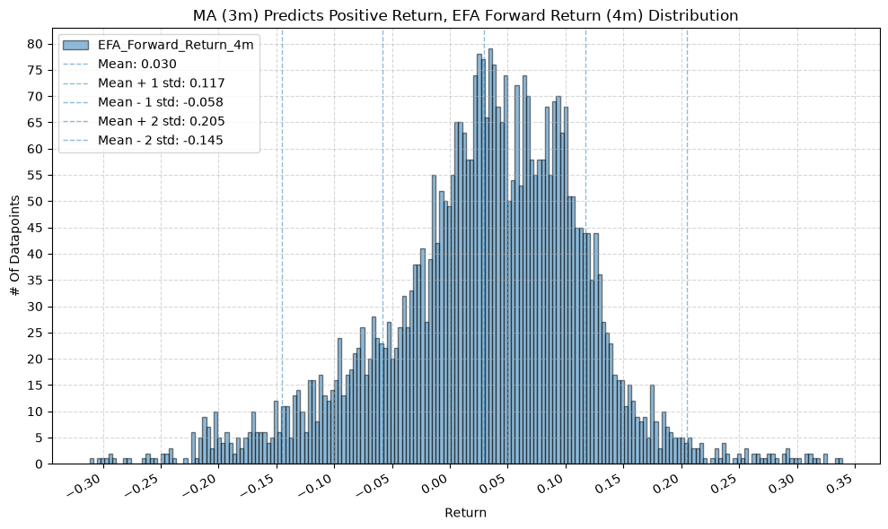
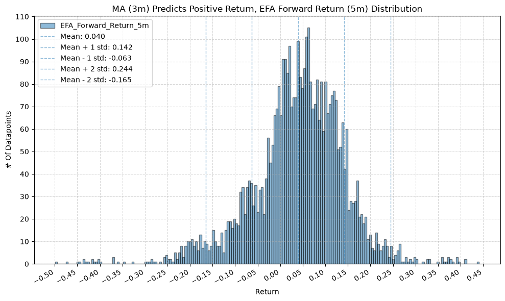
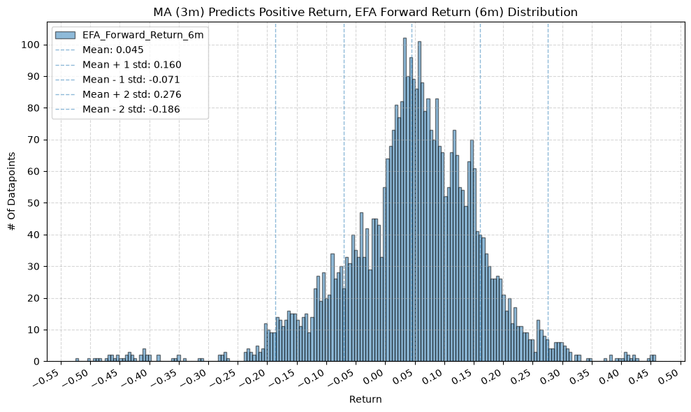
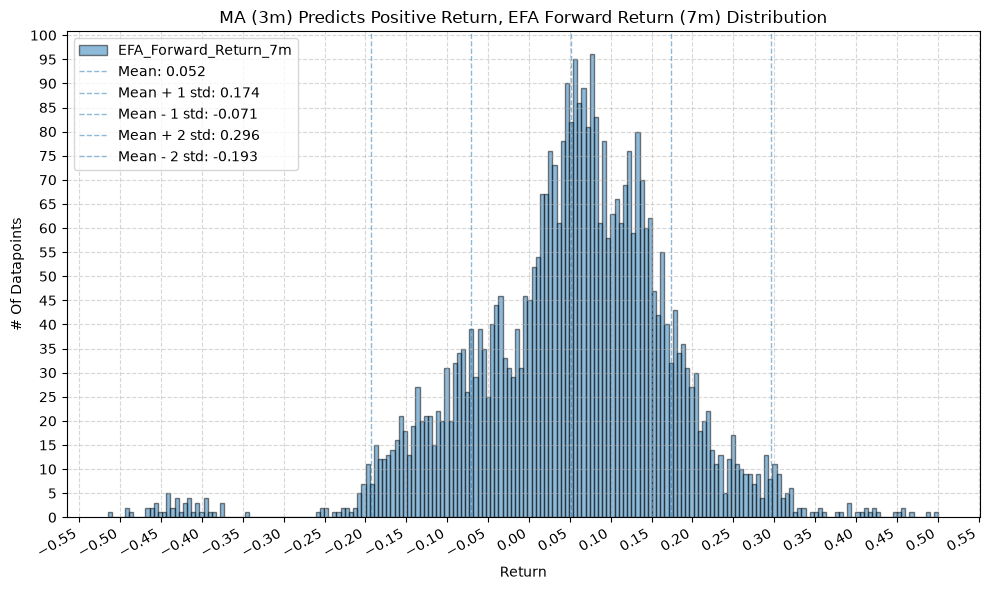
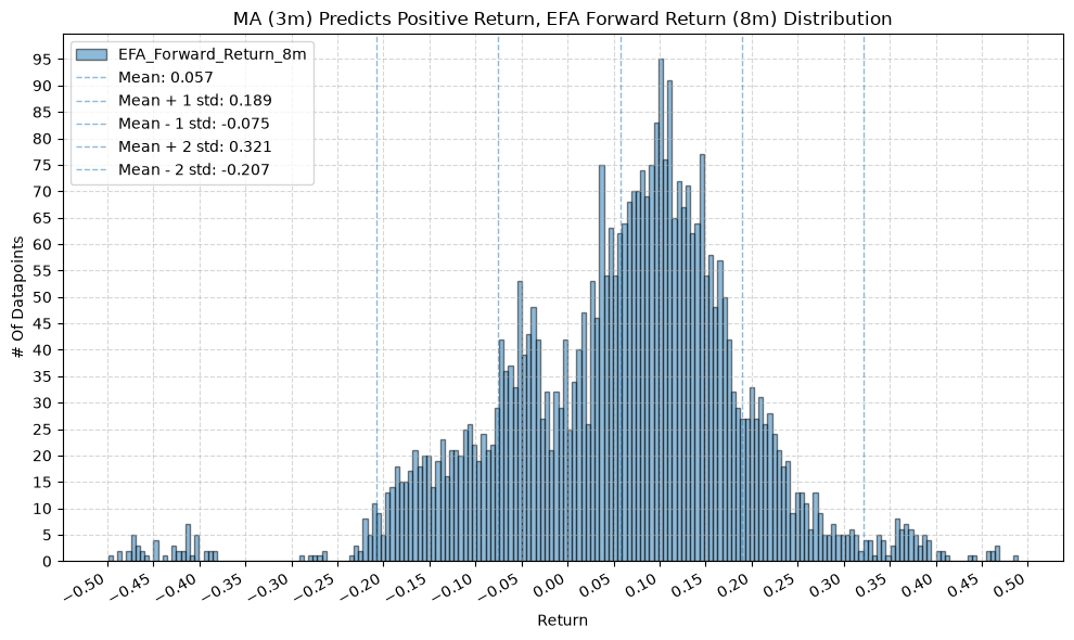
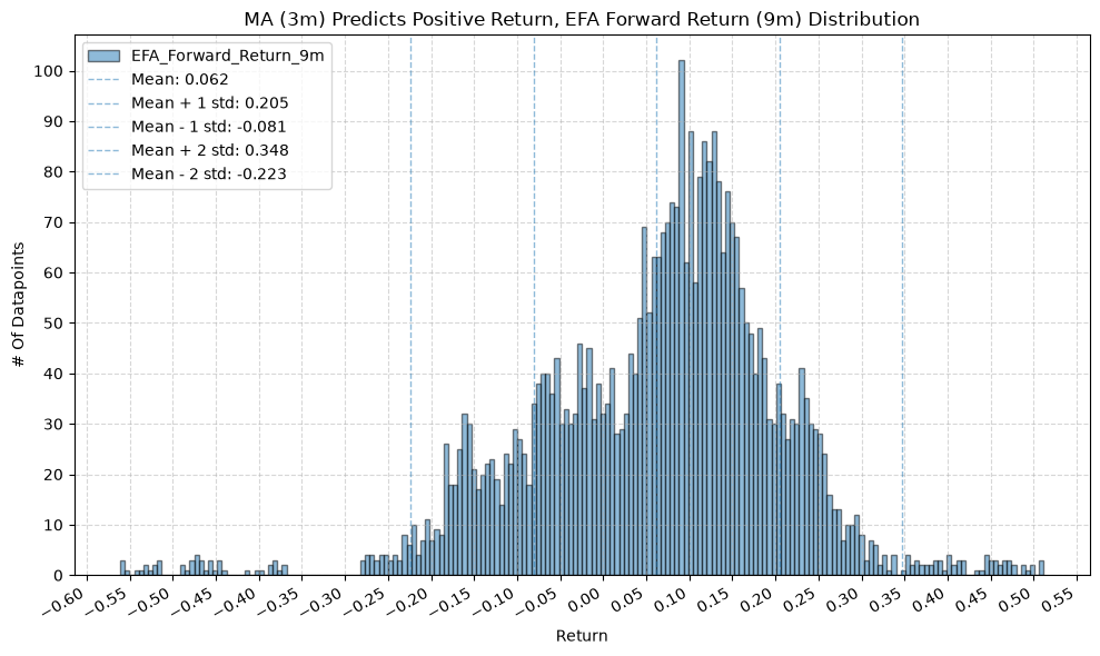
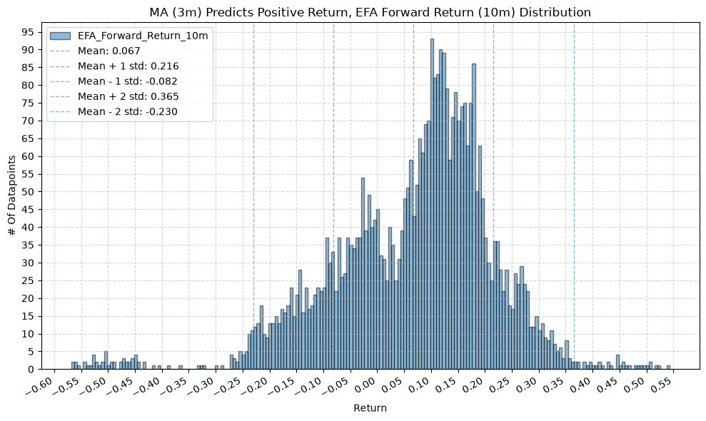
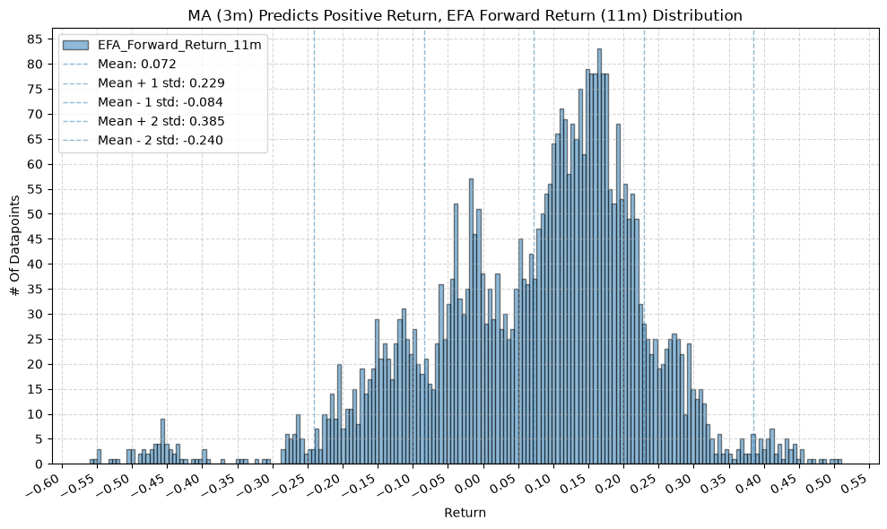
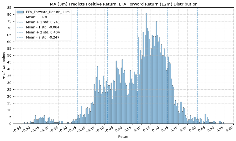
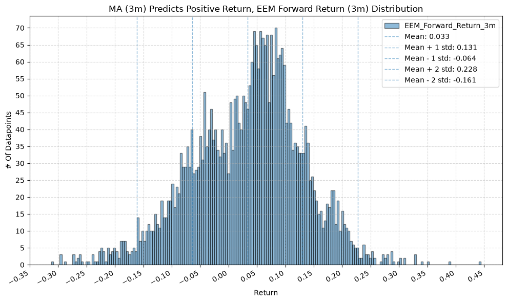
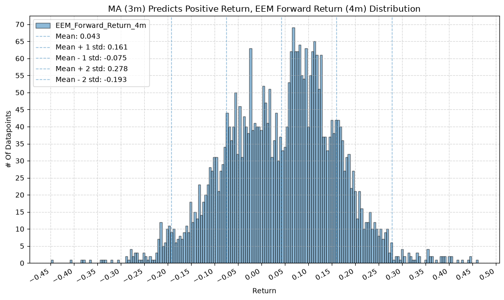
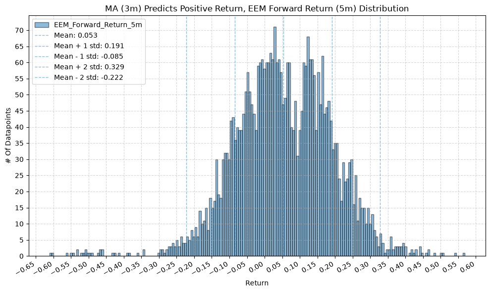
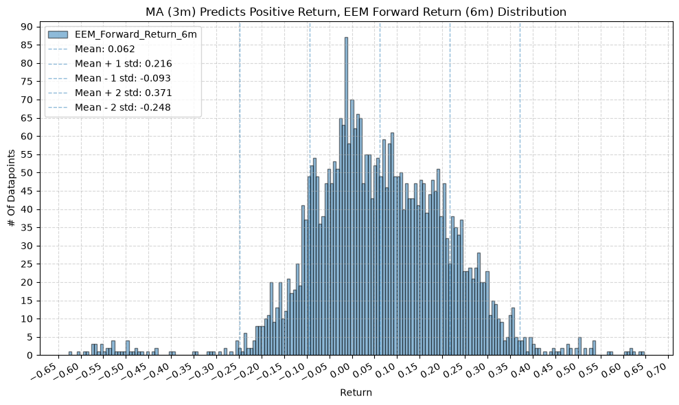
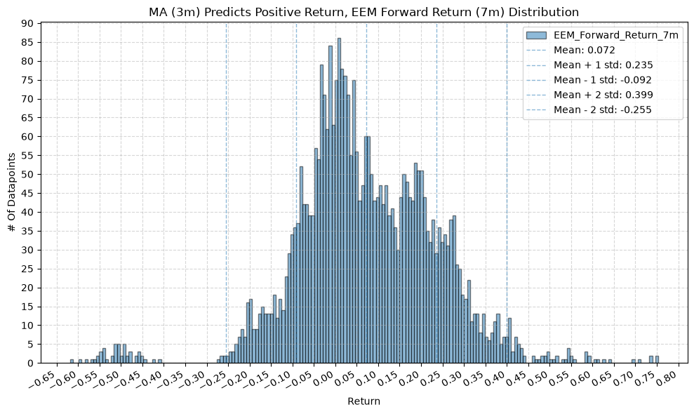
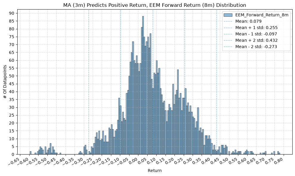
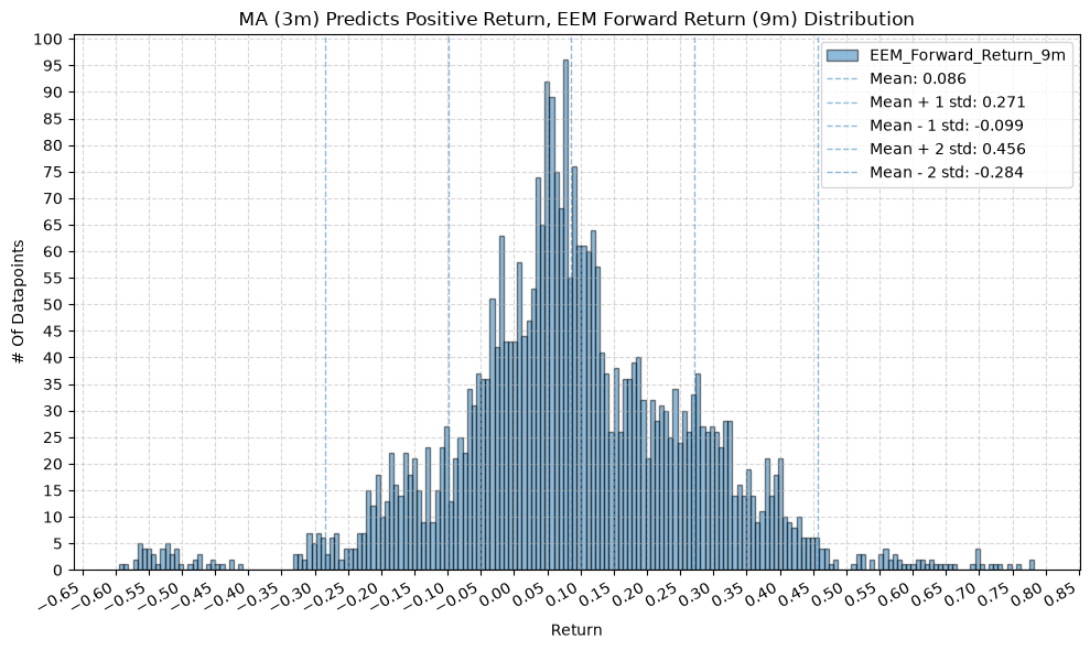
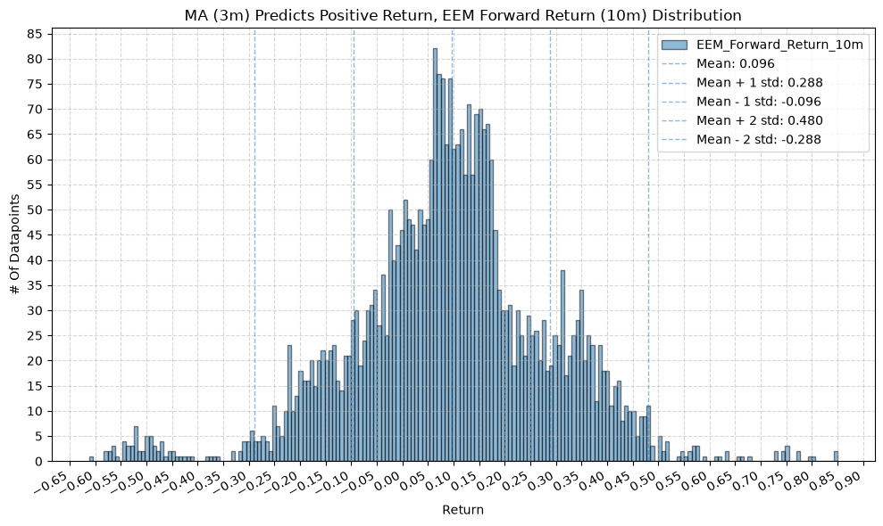
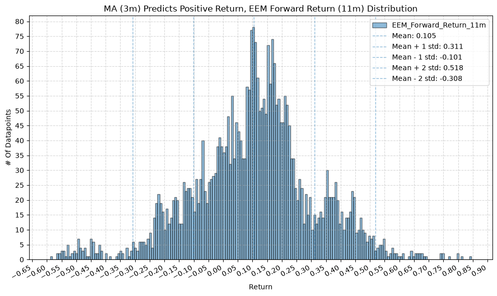
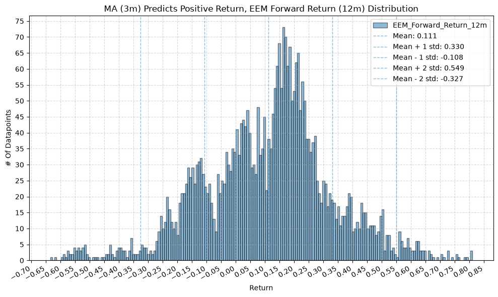
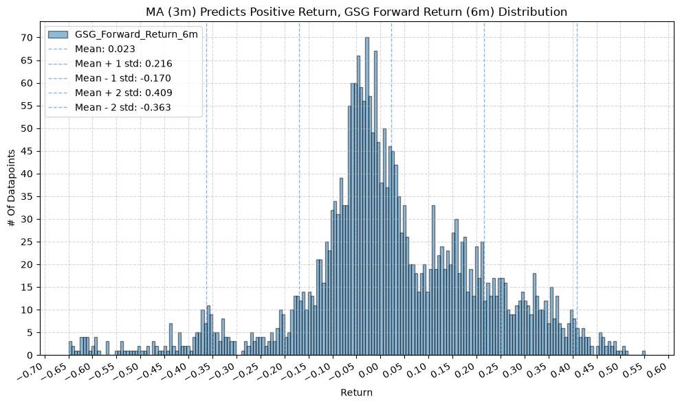
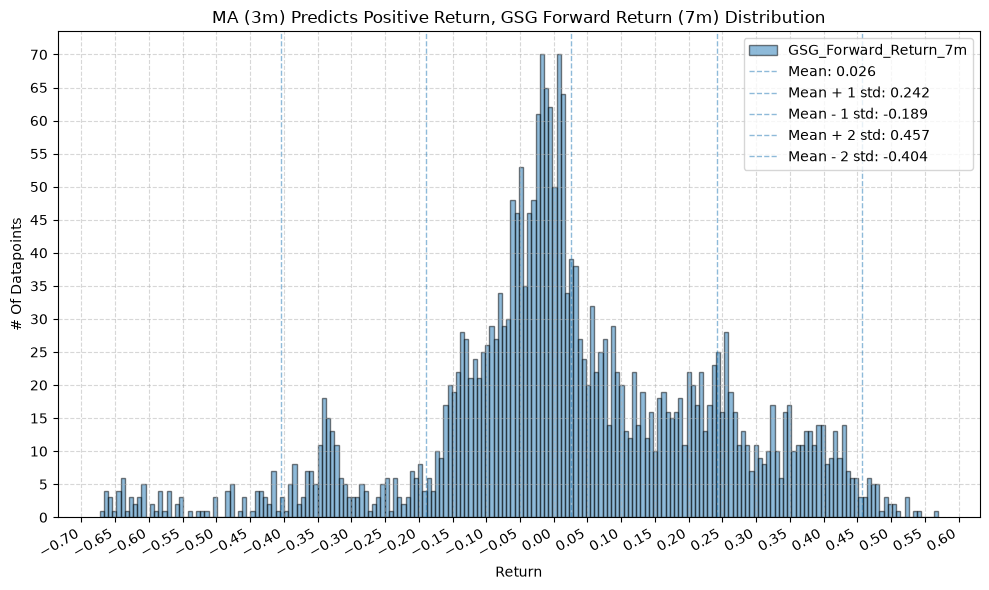
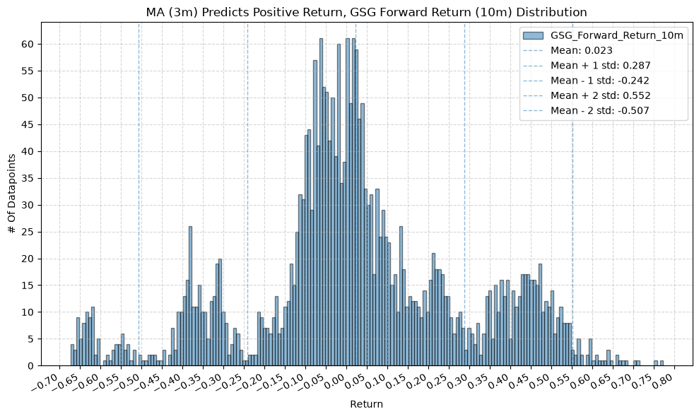
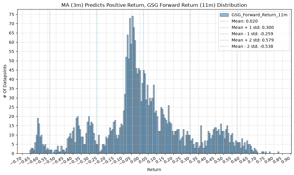
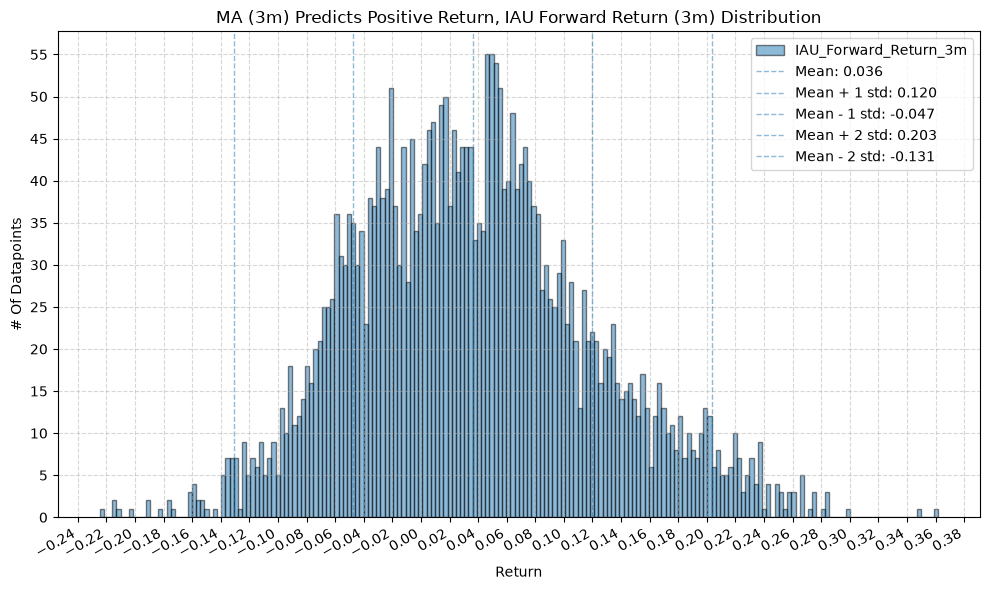
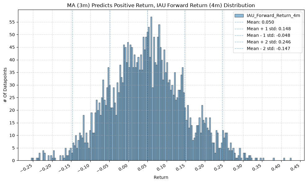
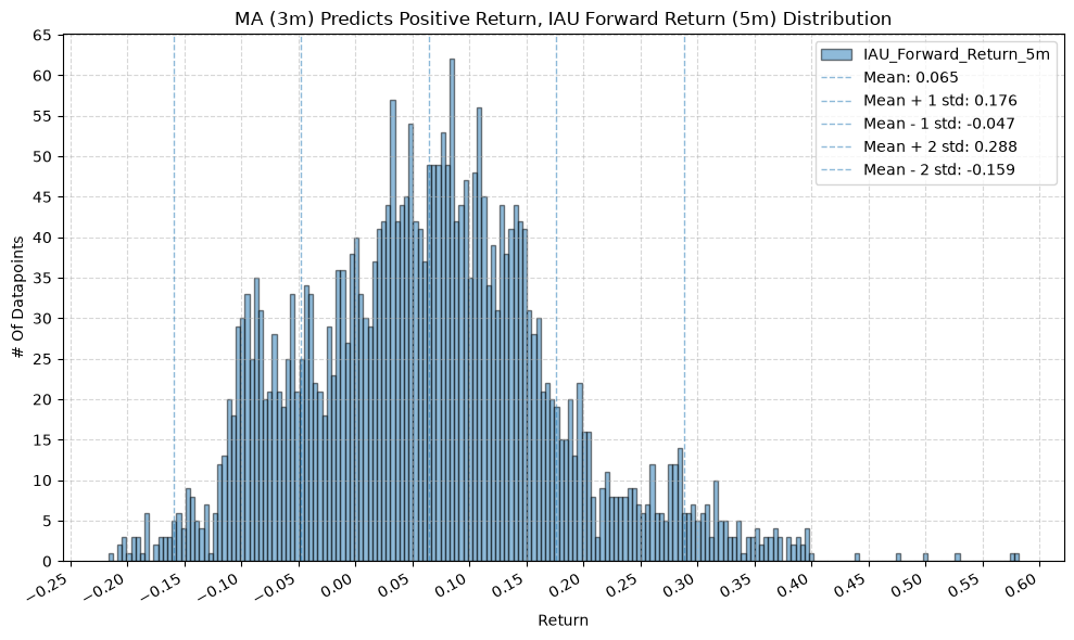
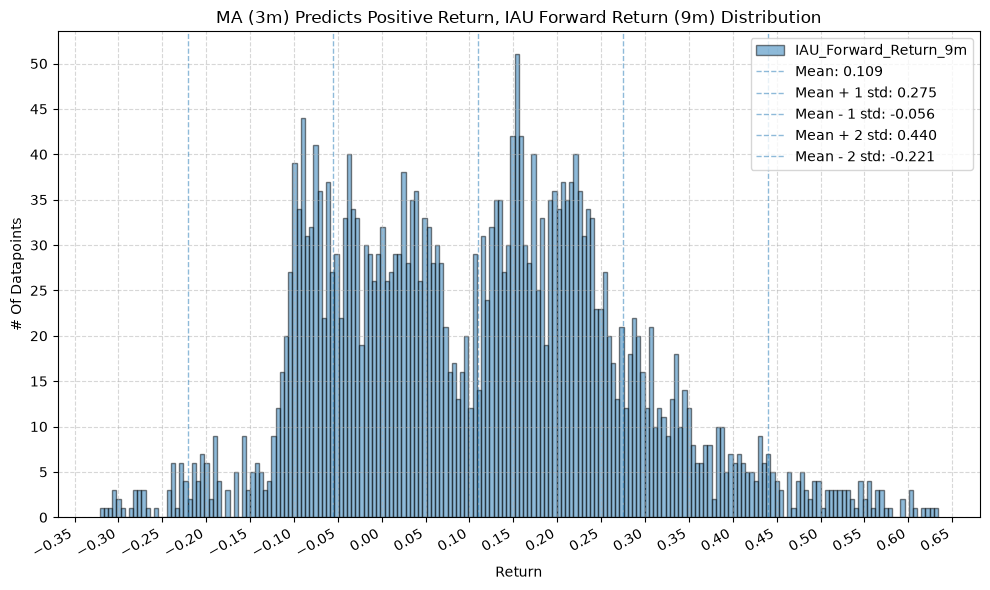
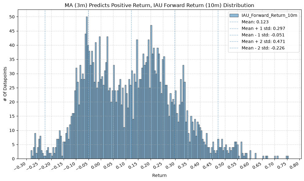
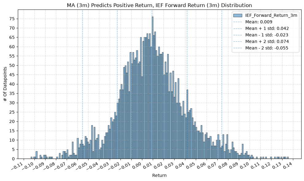
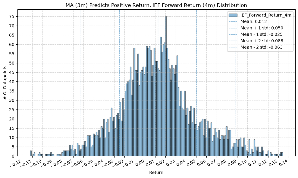
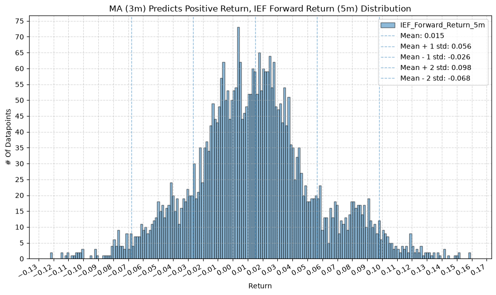
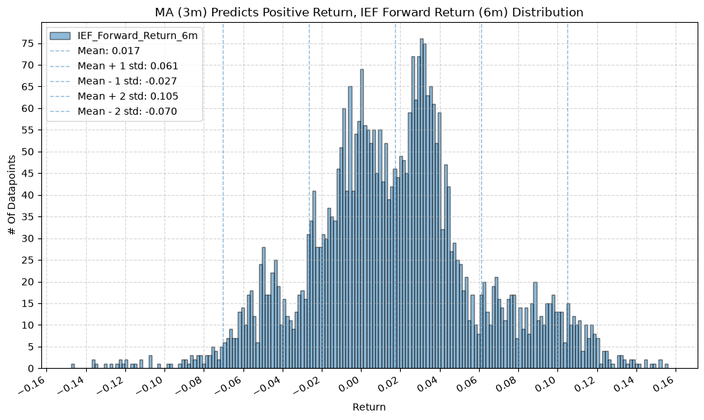
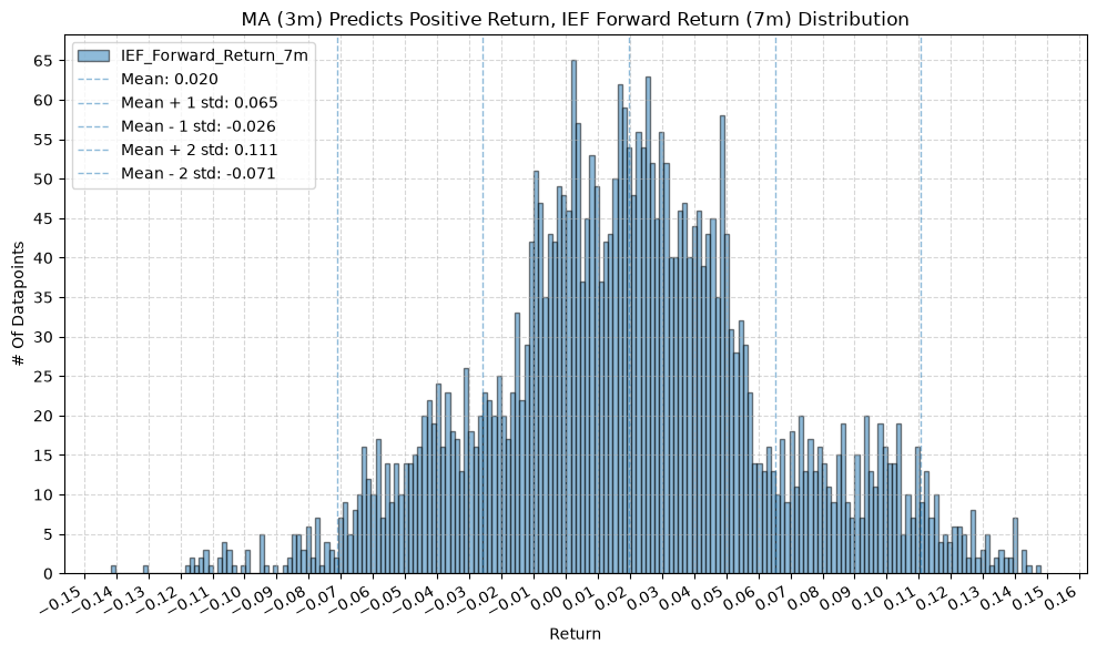
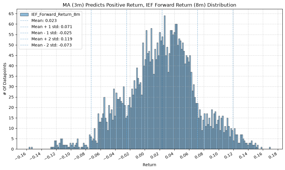
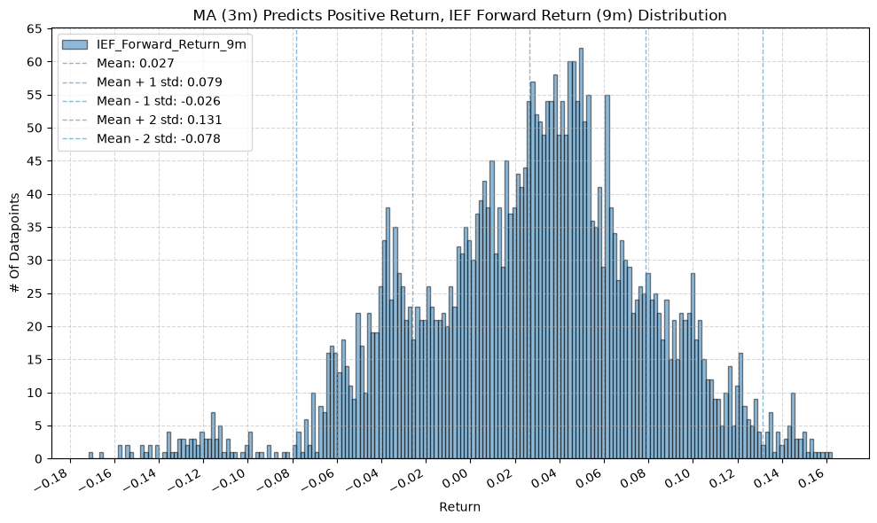
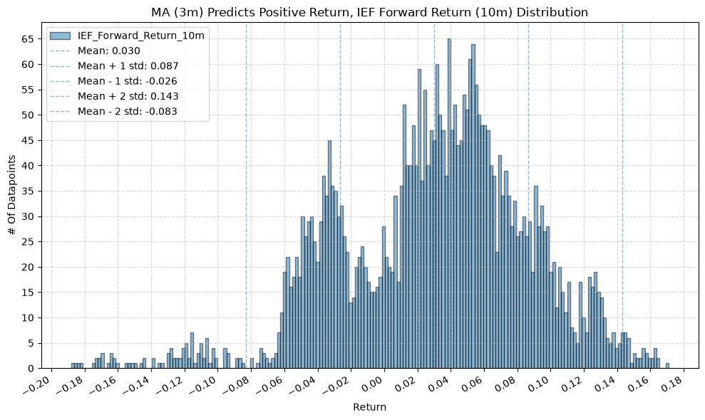
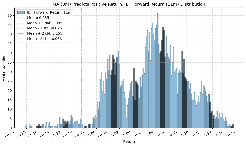
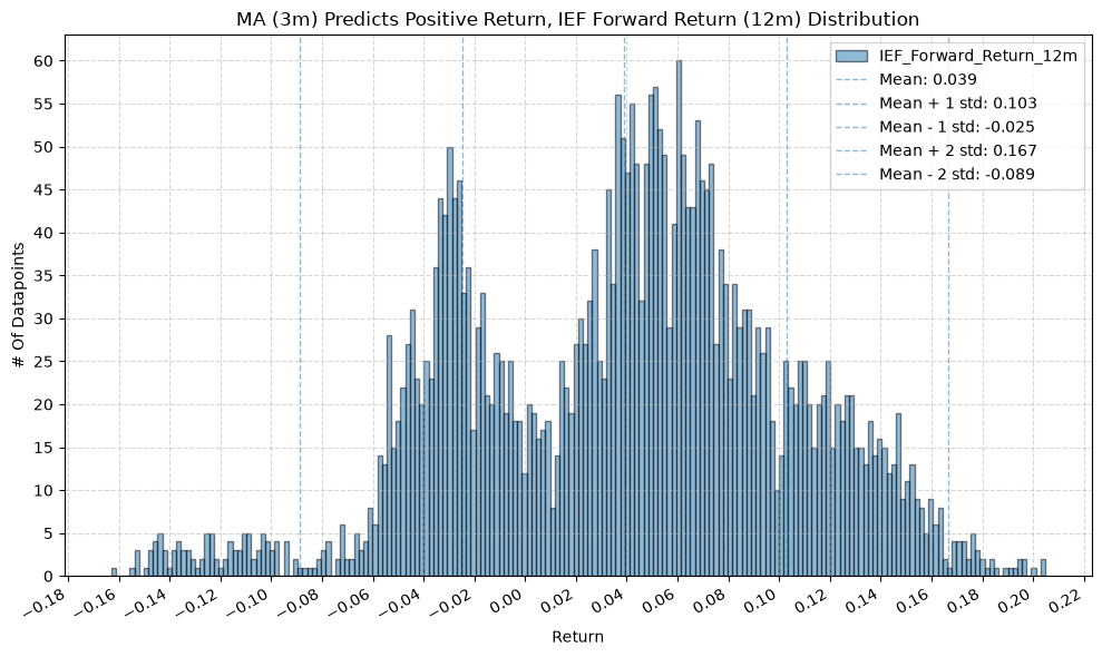
for fr_label, fr_window in forward_return_windows.items():
plot_histogram(
df=data[data[f"{fund}_MA_Prediction_{ma_label}"] == 1],
plot_columns=[f"{fund}_Forward_Return_{fr_label}"],
title=f"MA ({ma_label}) Predicts Positive Return, {fund} Forward Return ({fr_label}) Distribution",
x_label="Return",
x_tick_spacing="Auto",
x_tick_rotation=30,
y_label="# Of Datapoints",
y_tick_spacing="Auto",
y_tick_rotation=0,
grid=True,
legend=True,
export_plot=False,
plot_file_name=None,
)
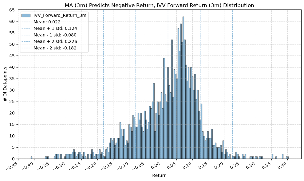
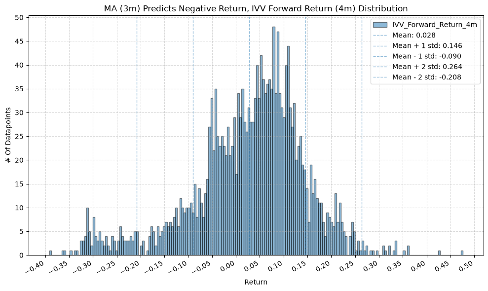
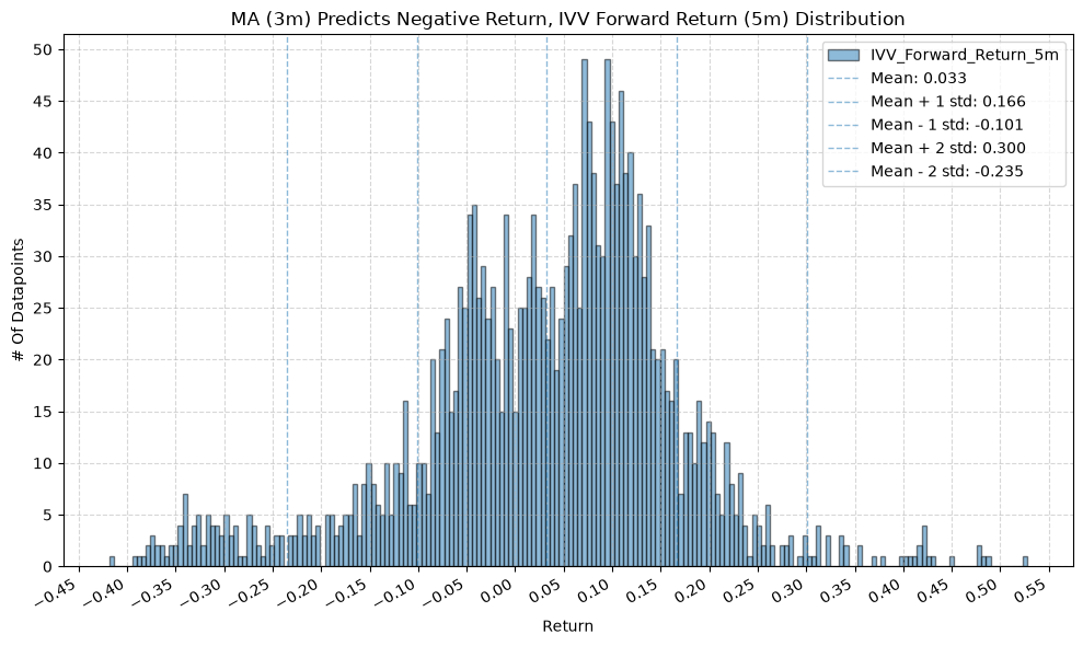
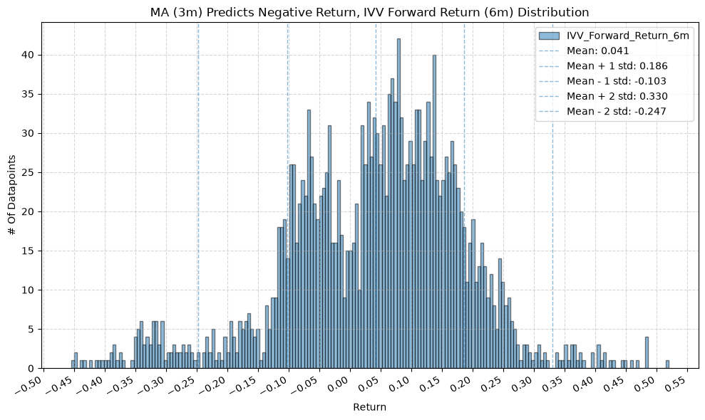
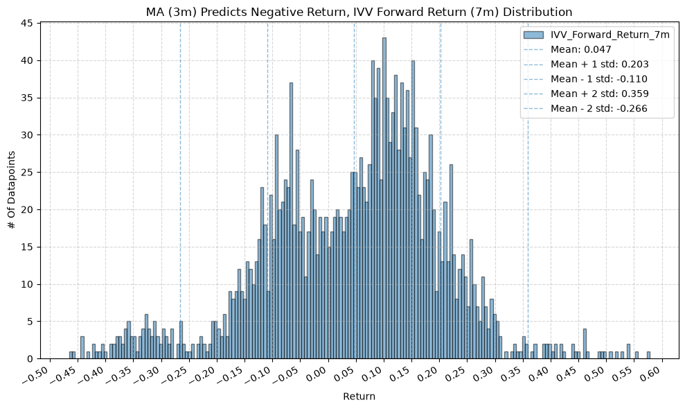
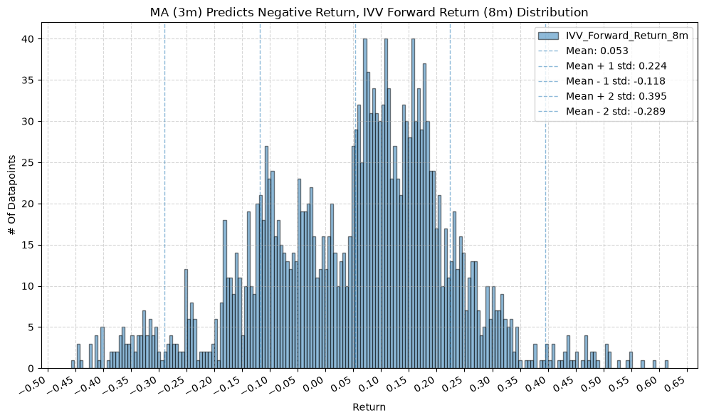
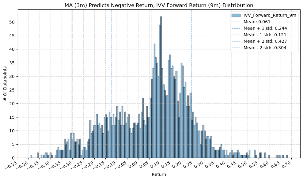
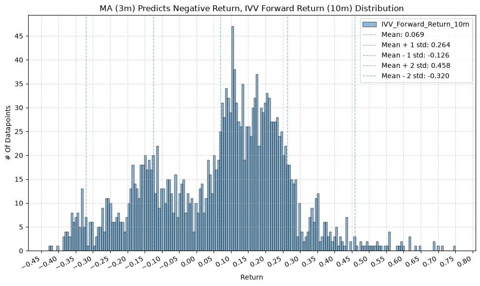
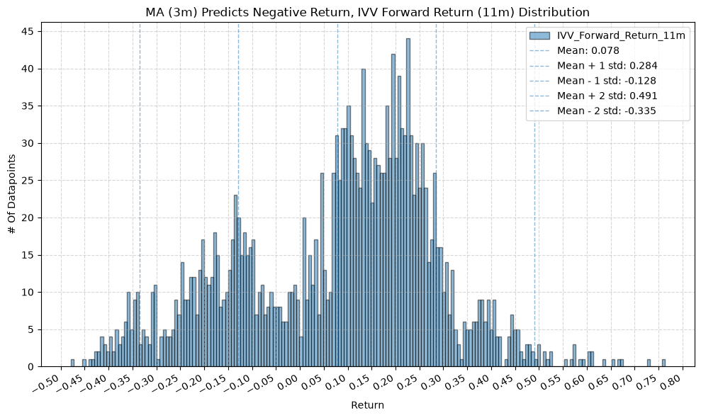
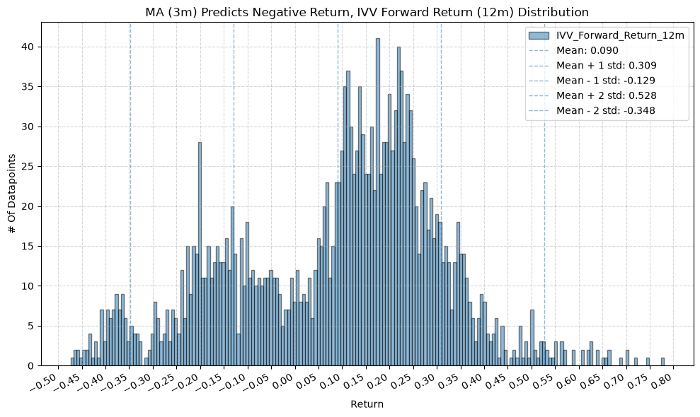
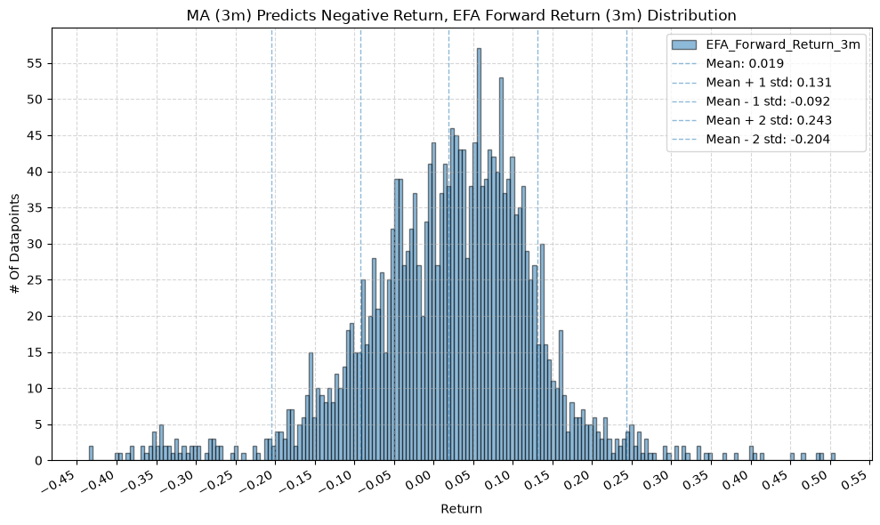
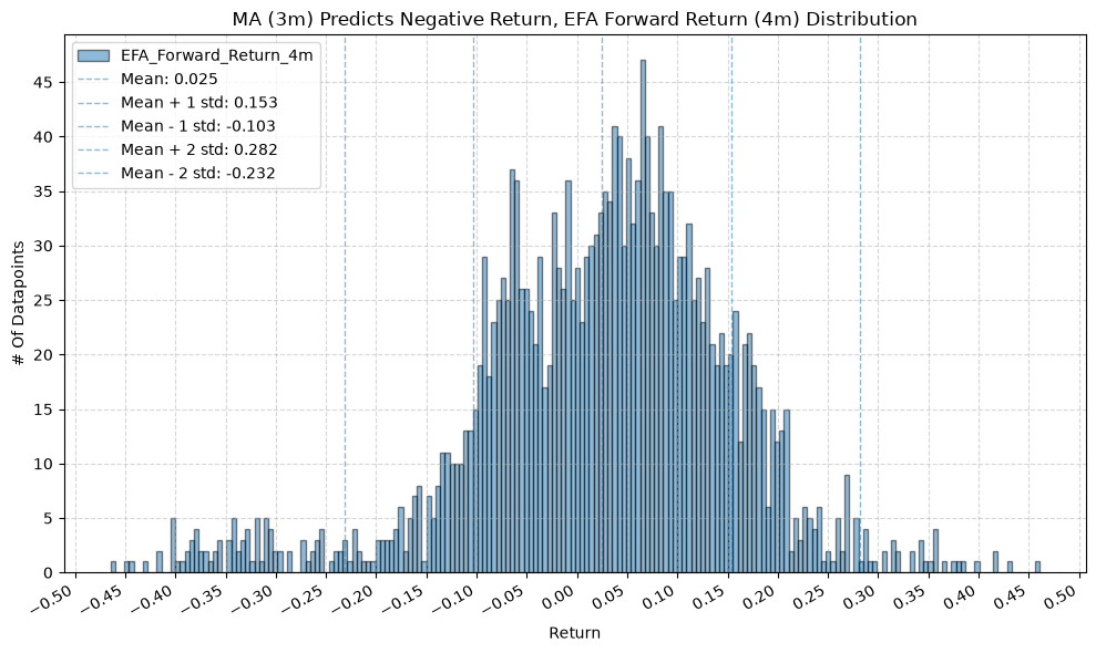
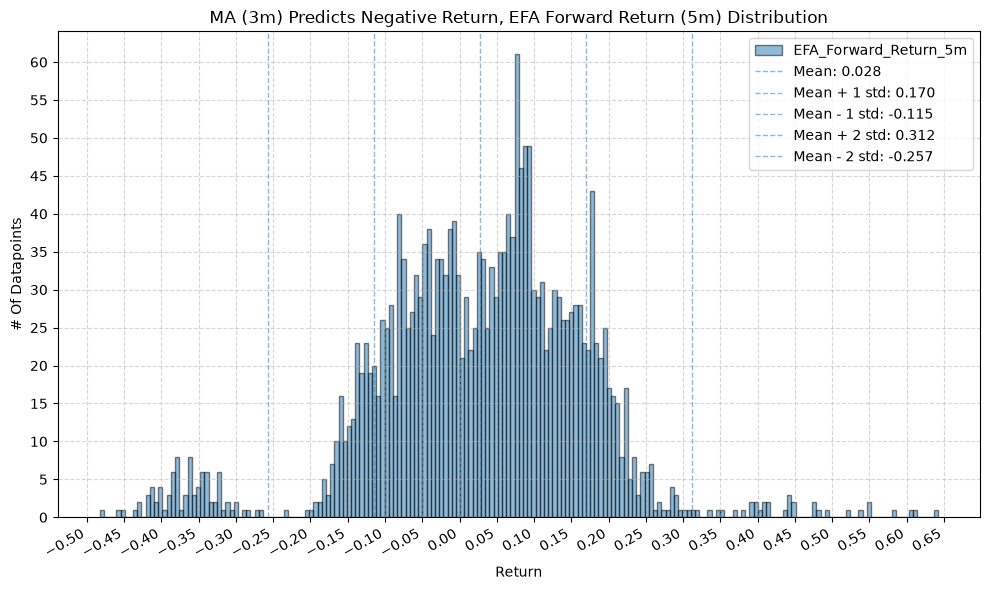
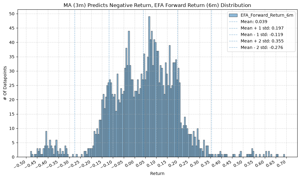
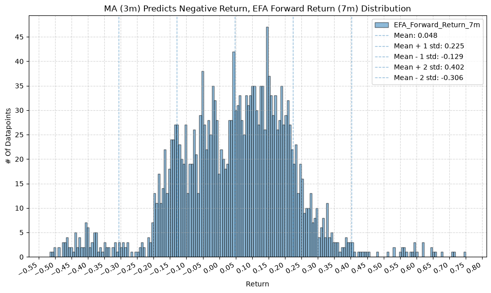
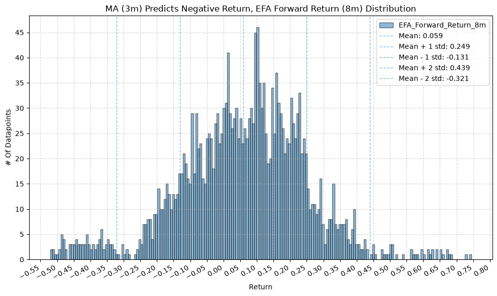
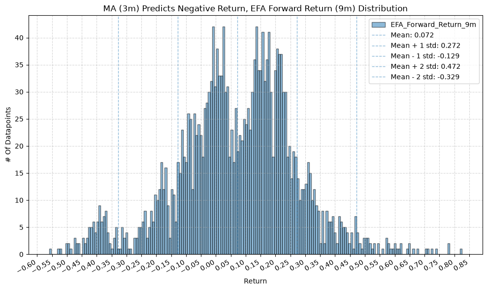
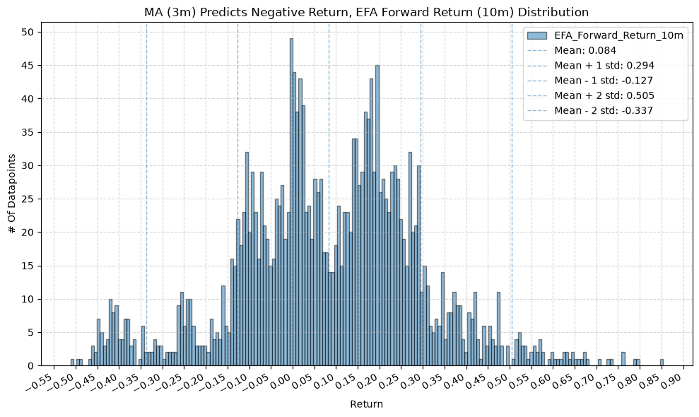
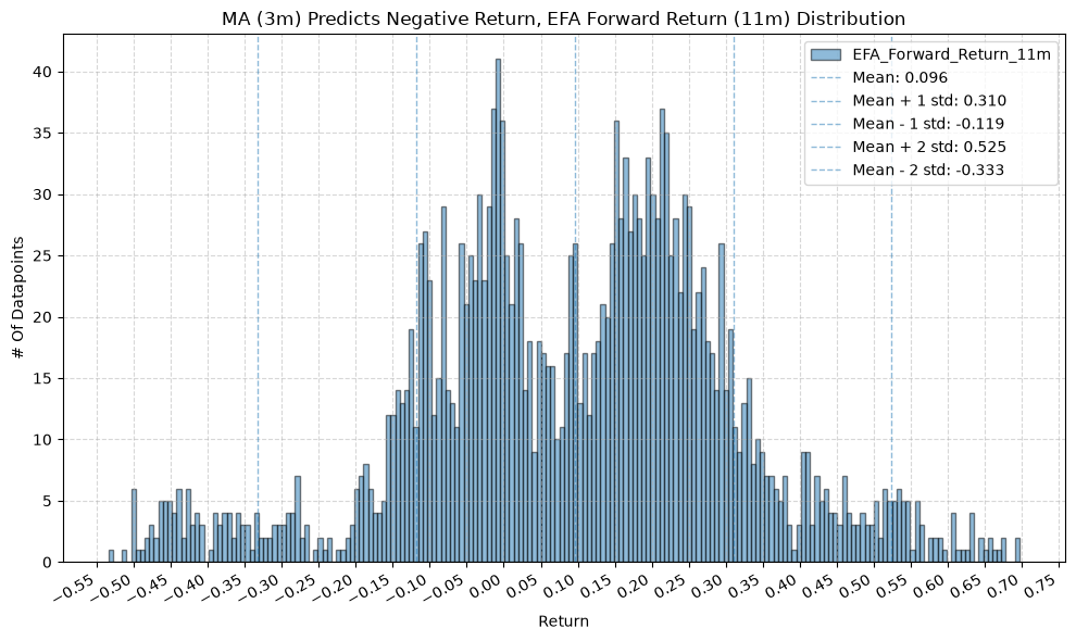
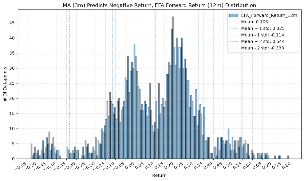
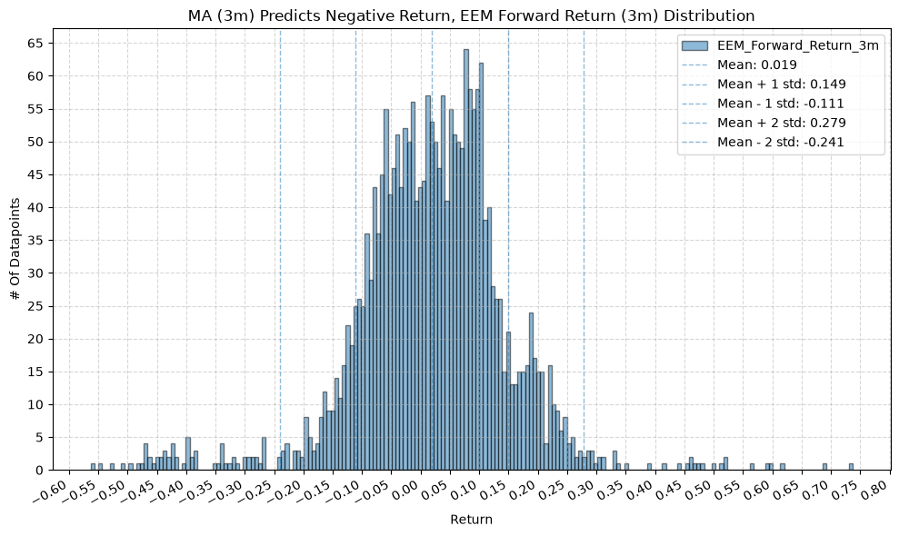
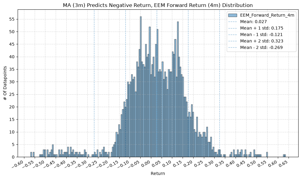
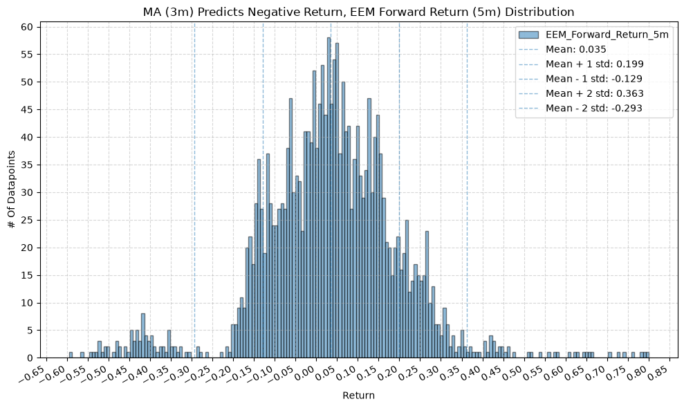
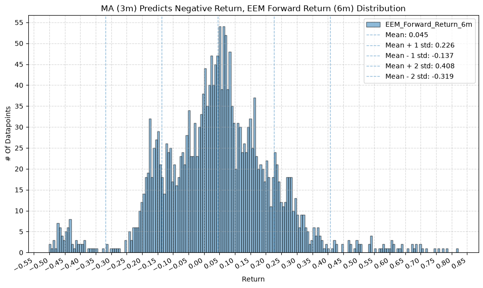
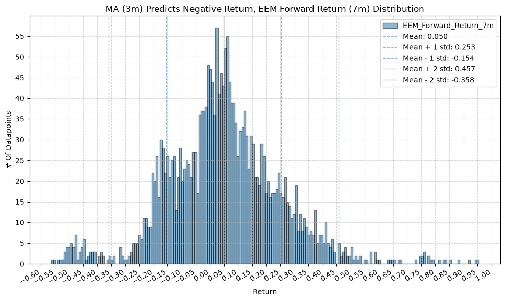
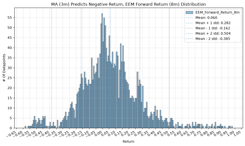
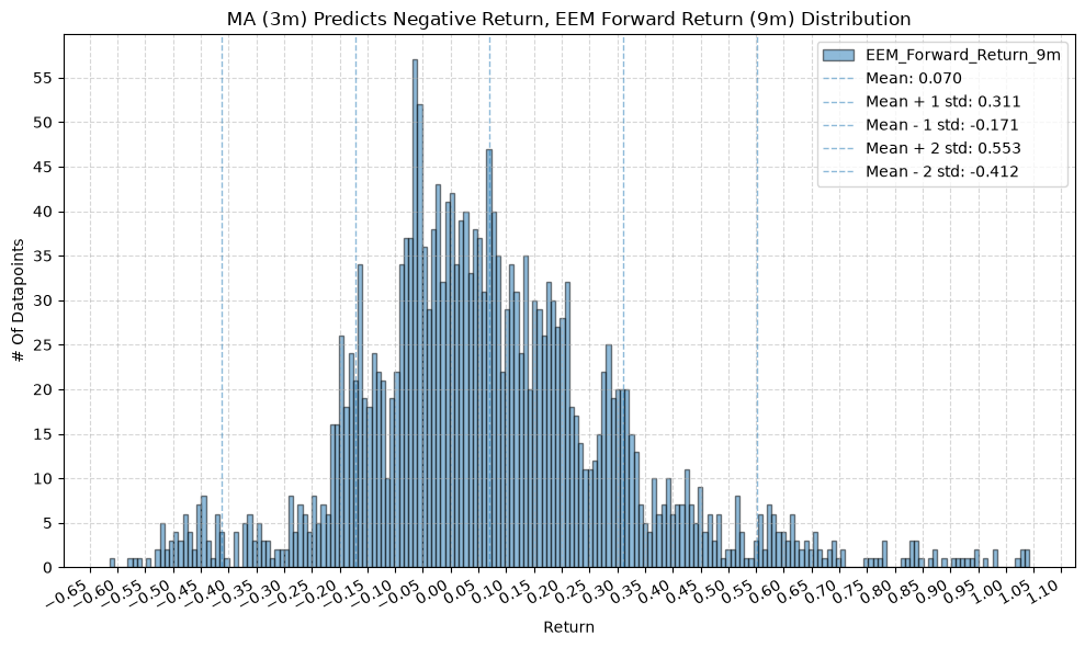
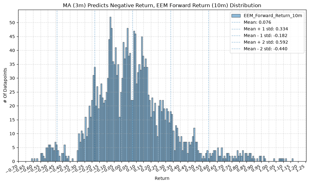
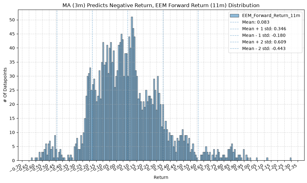
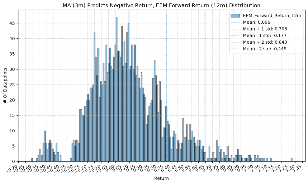
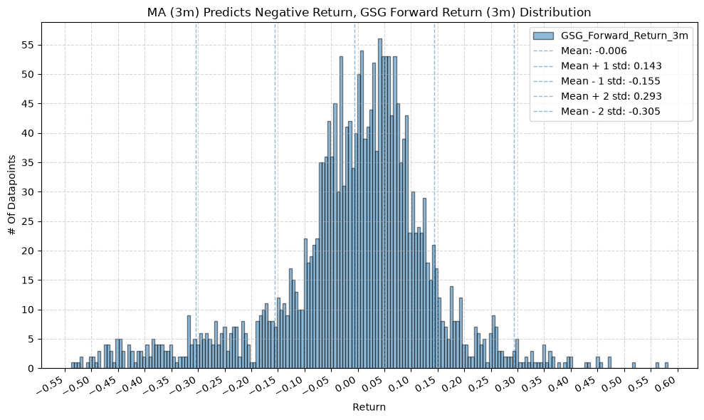
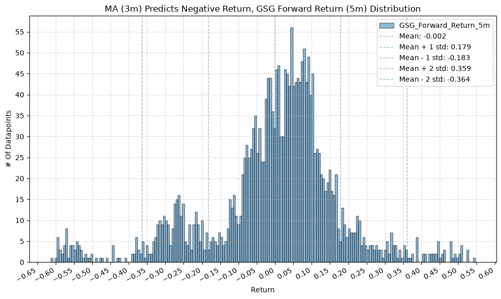
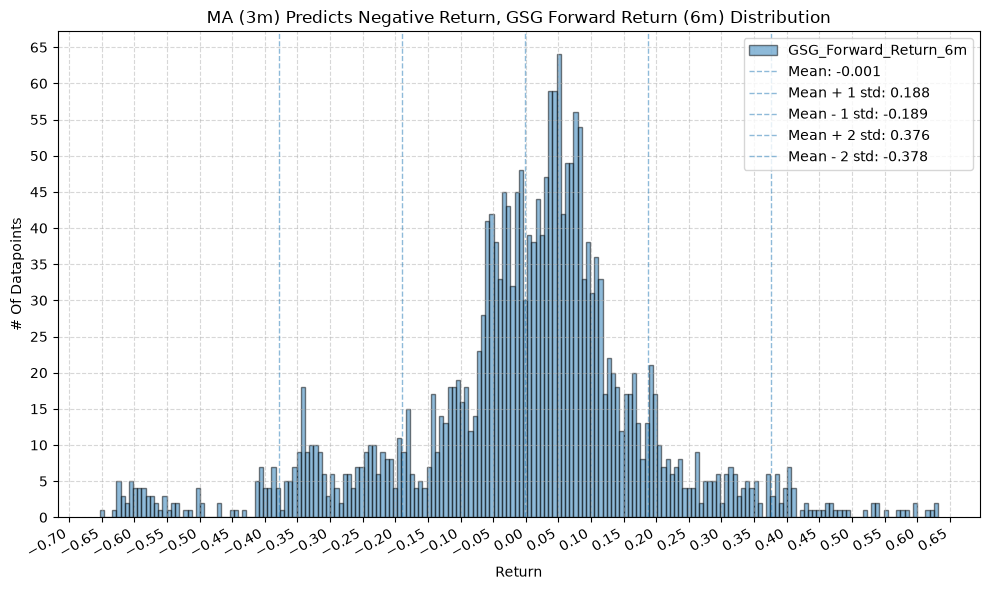
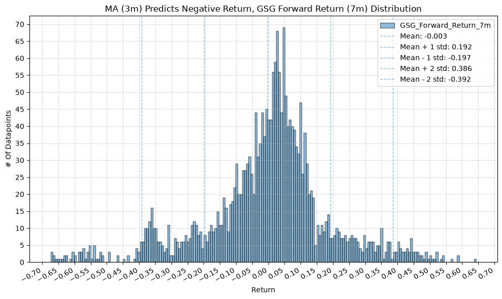
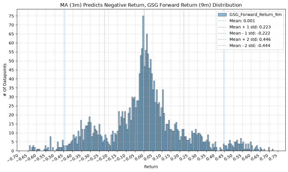
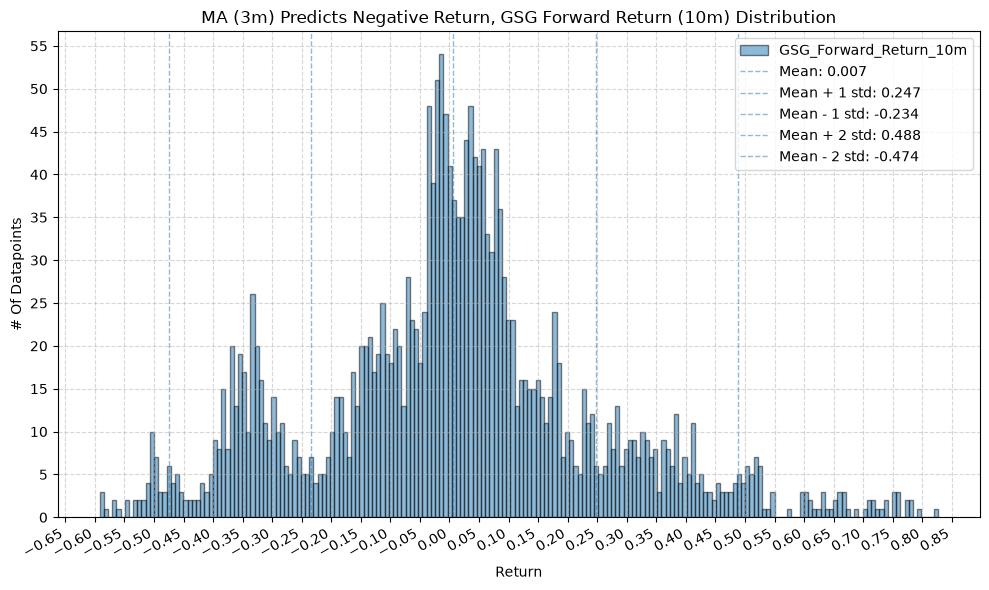
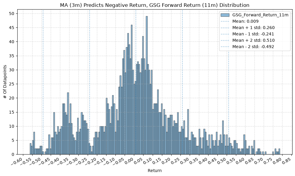
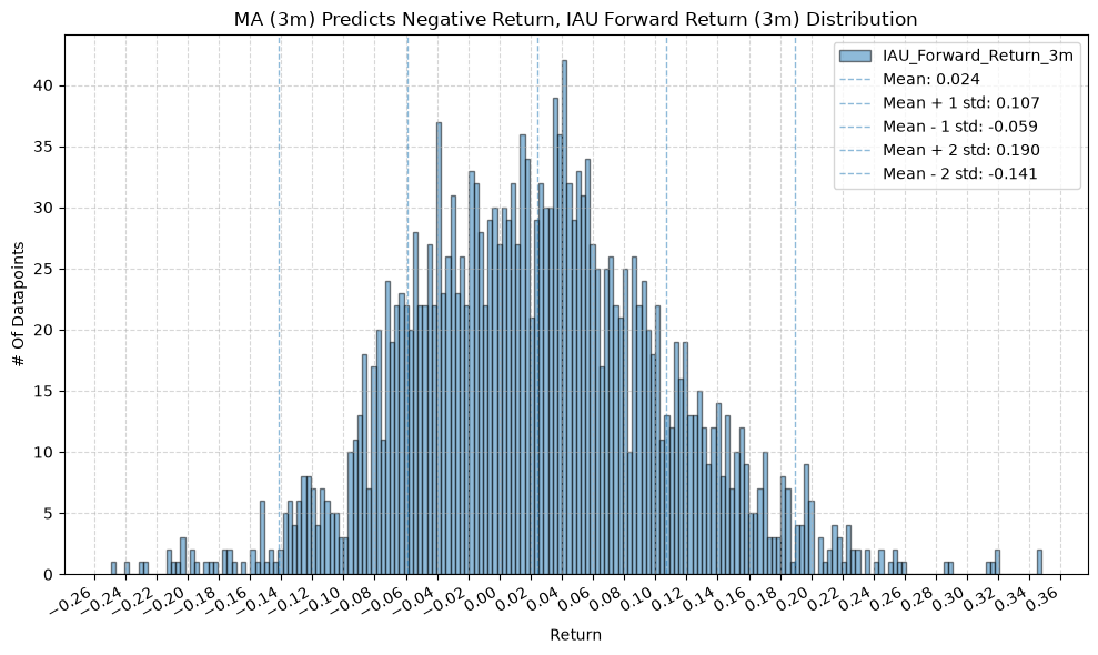
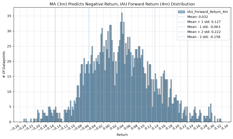
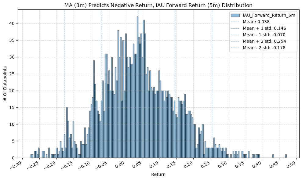
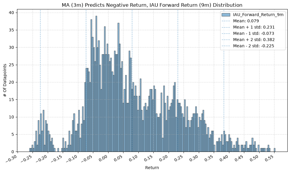
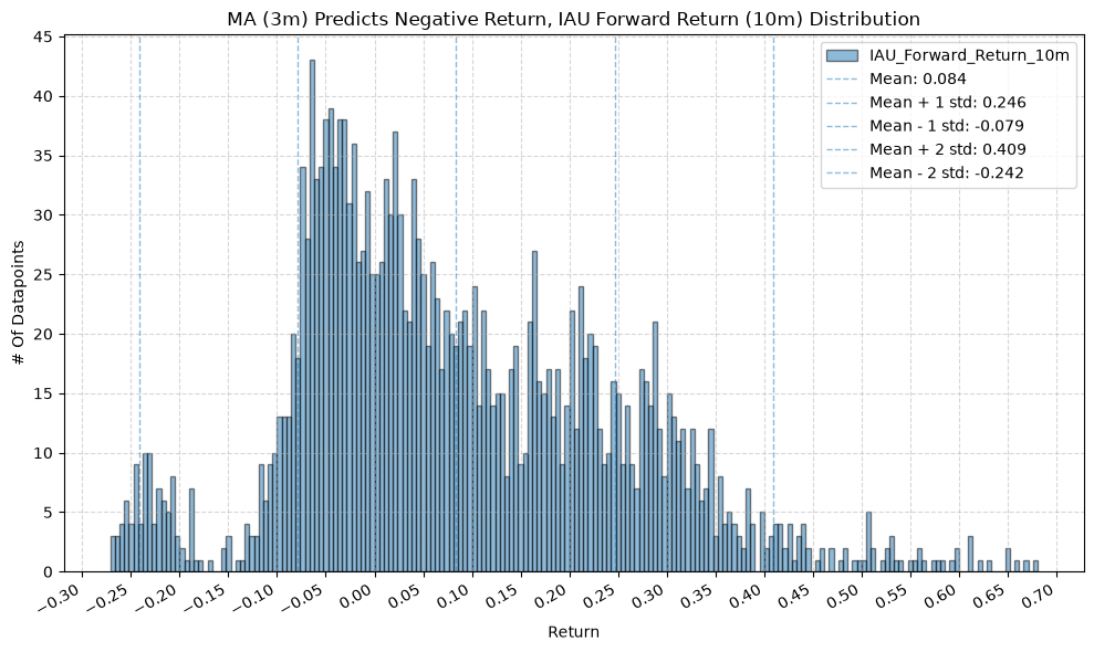
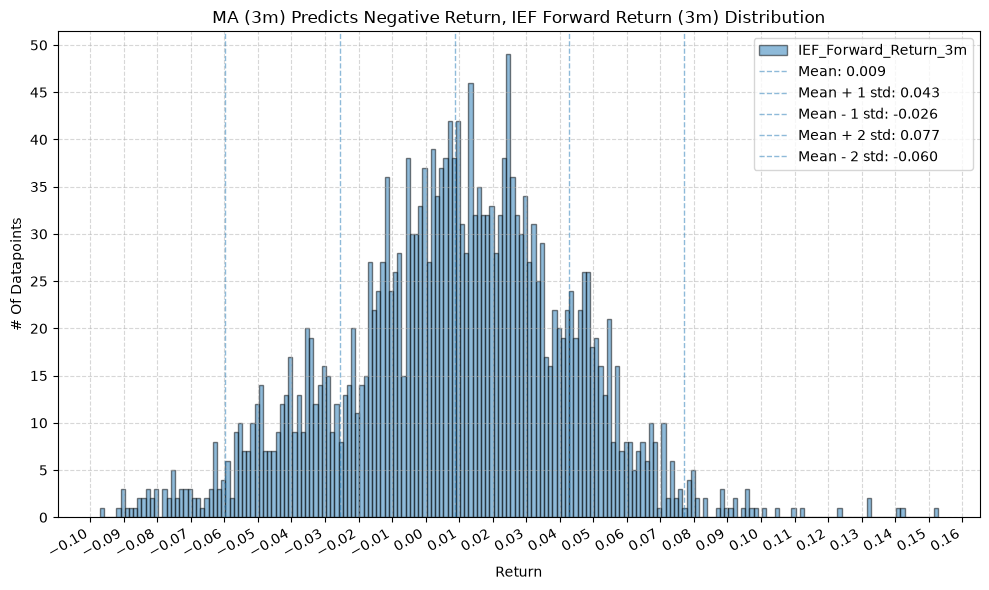
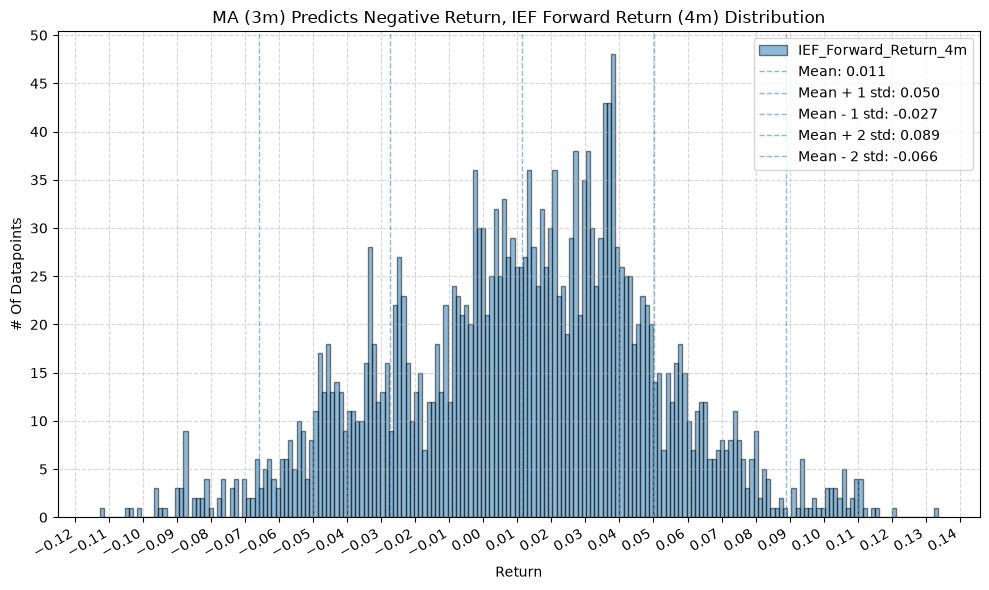
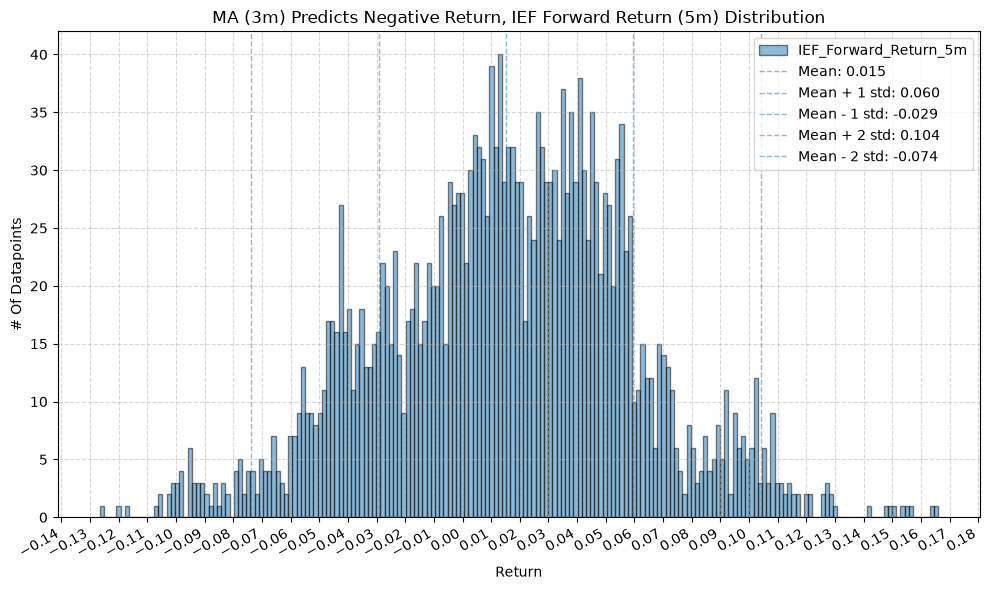
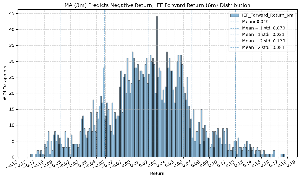
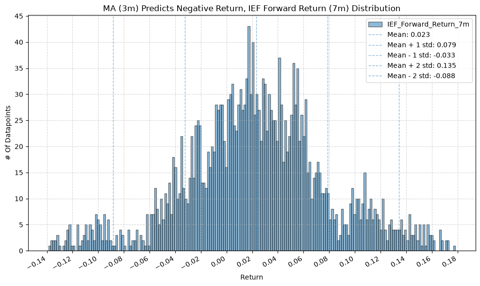
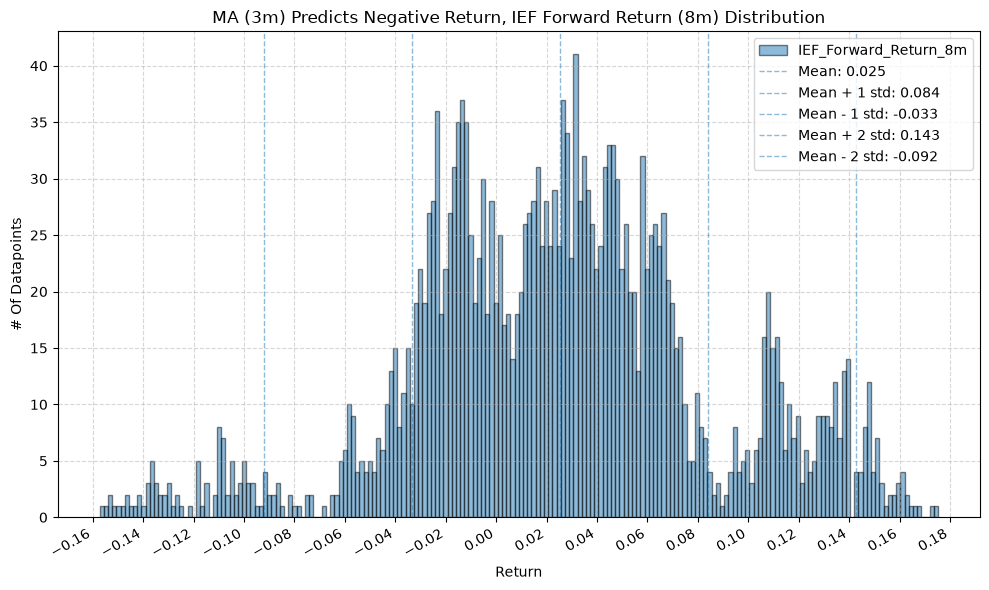
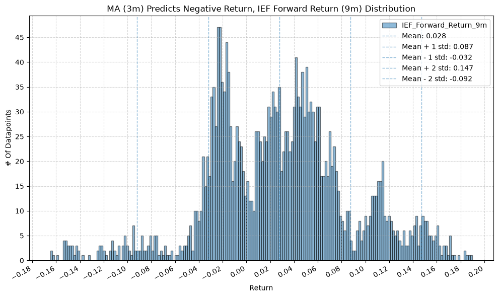
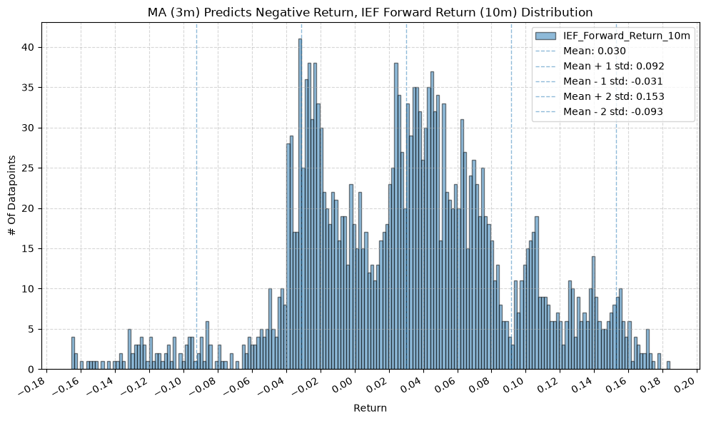
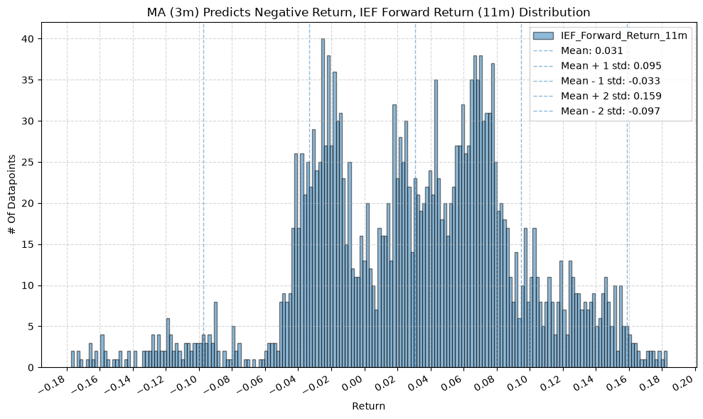
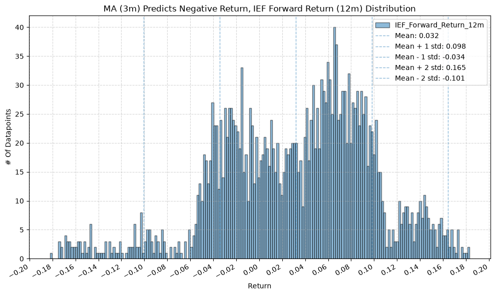
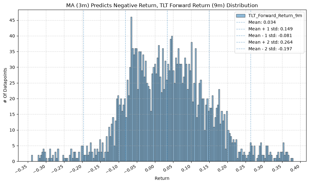
plot_histogram(
df=data[data[f"{fund}_MA_Prediction_{ma_label}"] == -1],
plot_columns=[f"{fund}_Forward_Return_{fr_label}"],
title=f"MA ({ma_label}) Predicts Negative Return, {fund} Forward Return ({fr_label}) Distribution",
x_label="Return",
x_tick_spacing="Auto",
x_tick_rotation=30,
y_label="# Of Datapoints",
y_tick_spacing="Auto",
y_tick_rotation=0,
grid=True,
legend=True,
export_plot=False,
plot_file_name=None,
)
GSG and IAU #
for fund, data in fund_data.items():
if fund not in ["GSG", "IAU"]:
continue
for ma_label, ma_window in ma_windows.items():
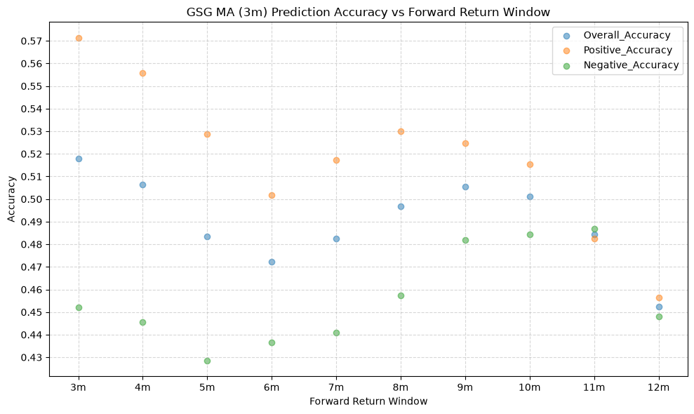
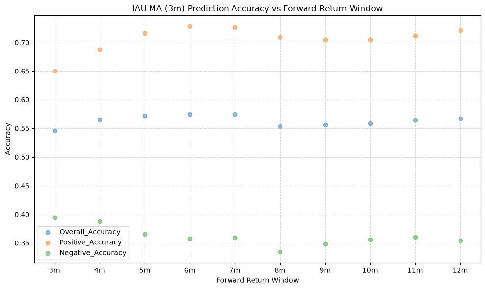
plot_scatter(
df=ma_prediction_results[(ma_prediction_results["Fund"] == fund) & (ma_prediction_results["MA_Window"] == ma_label)],
x_plot_column="Forward_Return_Window",
y_plot_columns=["Overall_Accuracy", "Positive_Accuracy", "Negative_Accuracy"],
title=f"{fund} MA ({ma_label}) Prediction Accuracy vs Forward Return Window",
x_label="Forward Return Window",
x_format="String",
x_format_decimal_places=0,
x_tick_spacing=1,
x_tick_start=None,
x_tick_rotation=0,
y_label="Accuracy",
y_format="Decimal",
y_format_decimal_places=2,
y_tick_spacing="Auto",
y_tick_rotation=0,
plot_OLS_regression_line=False,
OLS_column=None,
plot_Ridge_regression_line=False,
Ridge_column=None,
plot_RidgeCV_regression_line=False,
RidgeCV_column=None,
regression_constant=True,
grid=True,
legend=True,
export_plot=False,
plot_file_name=None,
)
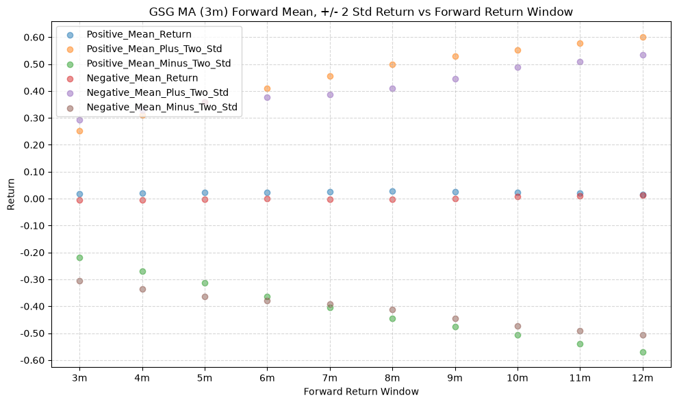
plot_scatter(
df=ma_prediction_results[(ma_prediction_results["Fund"] == fund) & (ma_prediction_results["MA_Window"] == ma_label)],
x_plot_column="Forward_Return_Window",
y_plot_columns=["Positive_Mean_Return", "Positive_Mean_Plus_Two_Std", "Positive_Mean_Minus_Two_Std", "Negative_Mean_Return", "Negative_Mean_Plus_Two_Std", "Negative_Mean_Minus_Two_Std"],
title=f"{fund} MA ({ma_label}) Forward Mean, +/- 2 Std Return vs Forward Return Window",
x_label="Forward Return Window",
x_format="String",
x_format_decimal_places=0,
x_tick_spacing=1,
x_tick_start=None,
x_tick_rotation=0,
y_label="Return",
y_format="Decimal",
y_format_decimal_places=2,
y_tick_spacing="Auto",
y_tick_rotation=0,
plot_OLS_regression_line=False,
OLS_column=None,
plot_Ridge_regression_line=False,
Ridge_column=None,
plot_RidgeCV_regression_line=False,
RidgeCV_column=None,
regression_constant=True,
grid=True,
legend=True,
export_plot=False,
plot_file_name=None,
)
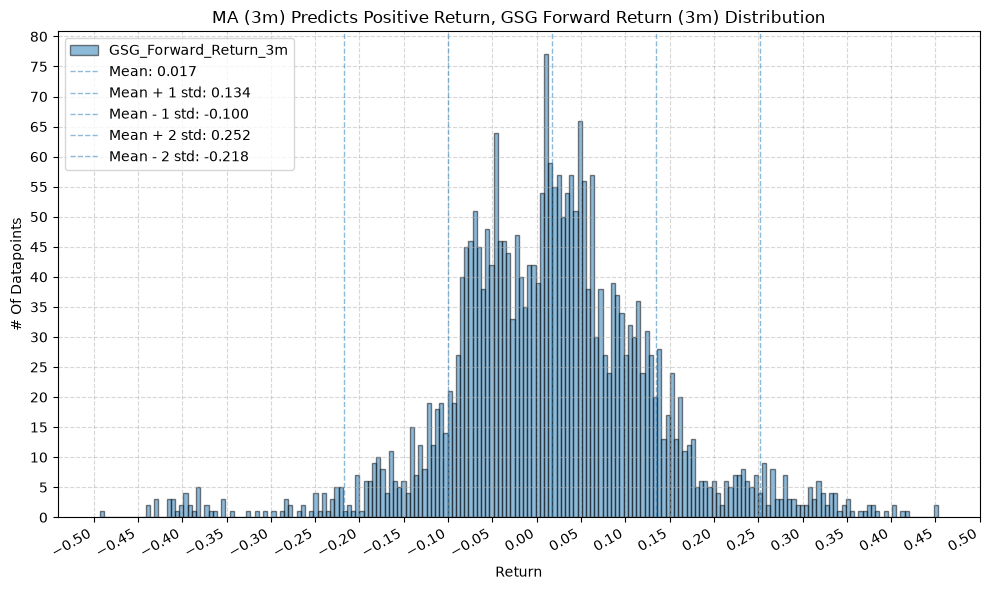
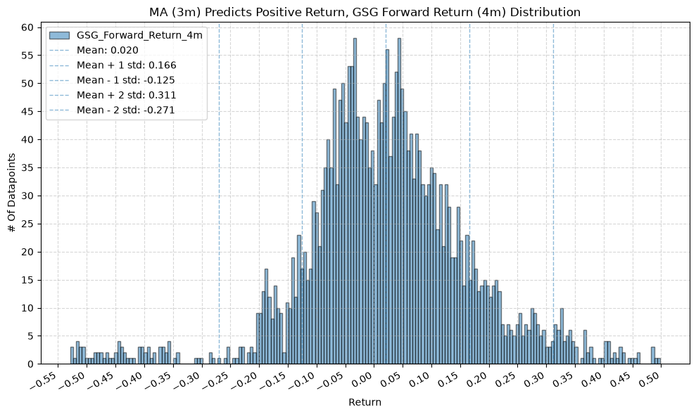
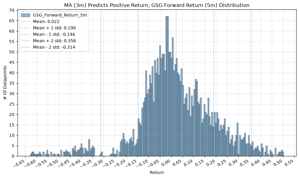
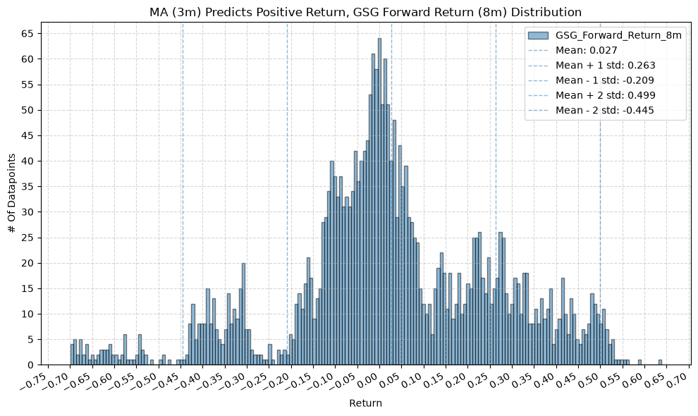
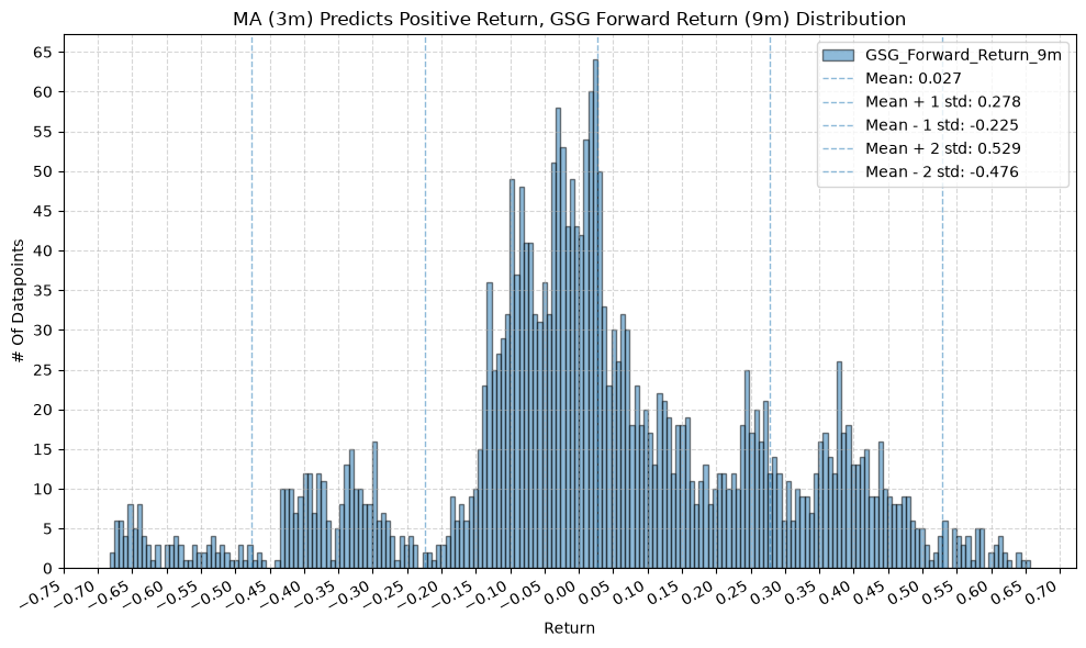
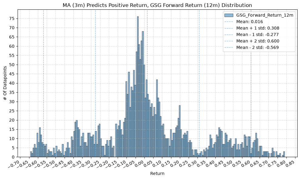
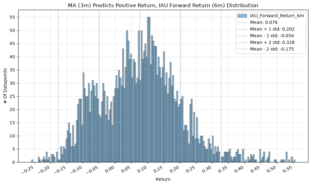
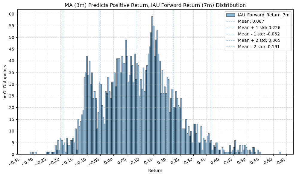
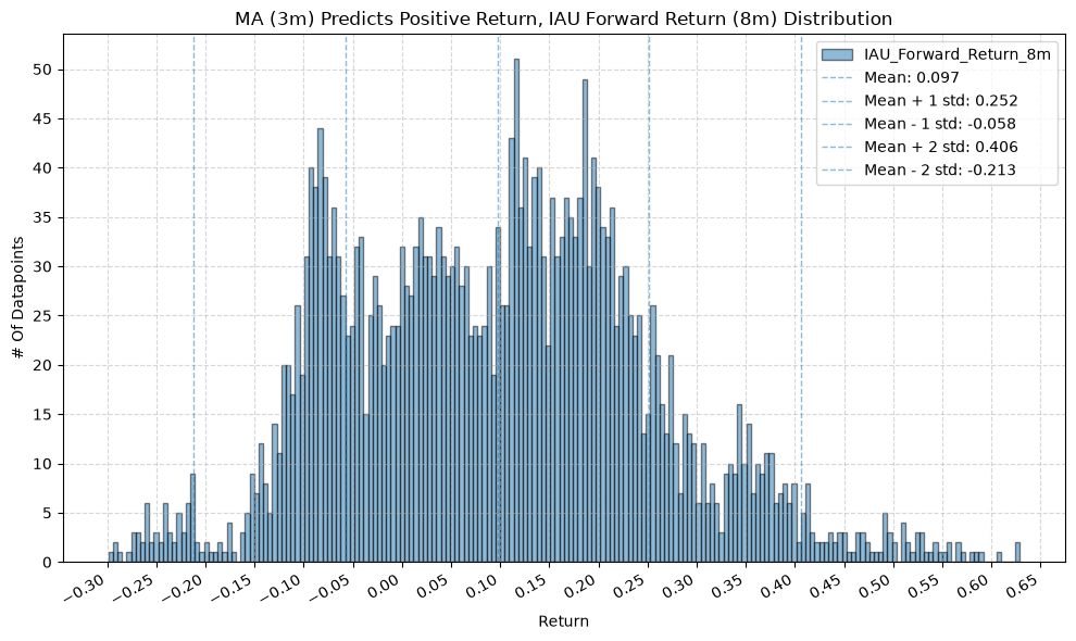
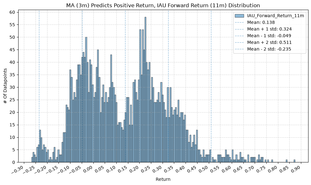
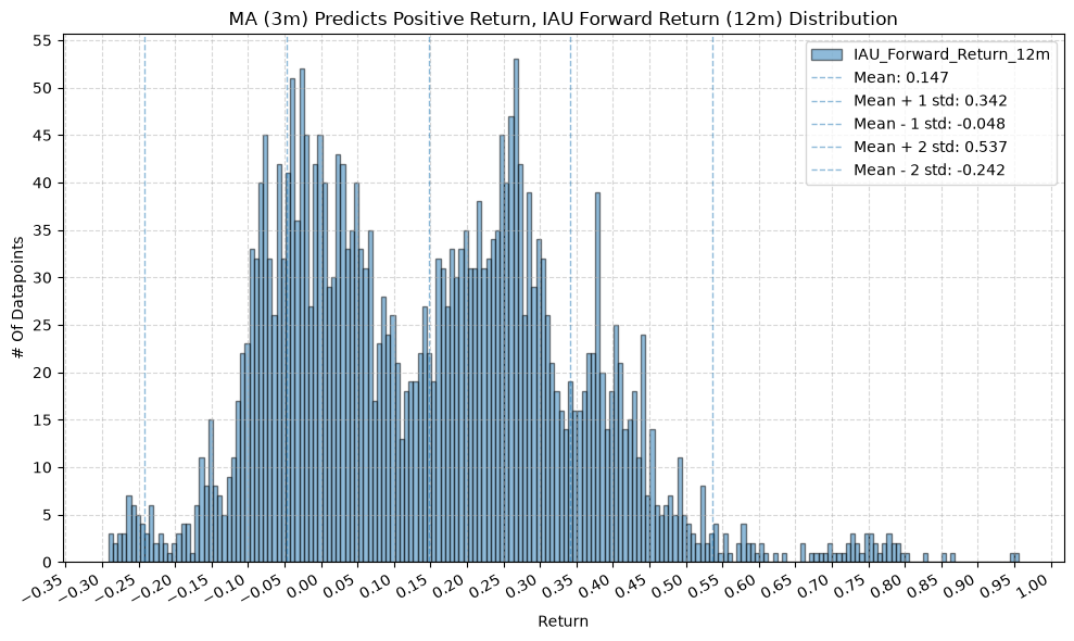
for fr_label, fr_window in forward_return_windows.items():
plot_histogram(
df=data[data[f"{fund}_MA_Prediction_{ma_label}"] == 1],
plot_columns=[f"{fund}_Forward_Return_{fr_label}"],
title=f"MA ({ma_label}) Predicts Positive Return, {fund} Forward Return ({fr_label}) Distribution",
x_label="Return",
x_tick_spacing="Auto",
x_tick_rotation=30,
y_label="# Of Datapoints",
y_tick_spacing="Auto",
y_tick_rotation=0,
grid=True,
legend=True,
export_plot=False,
plot_file_name=None,
)
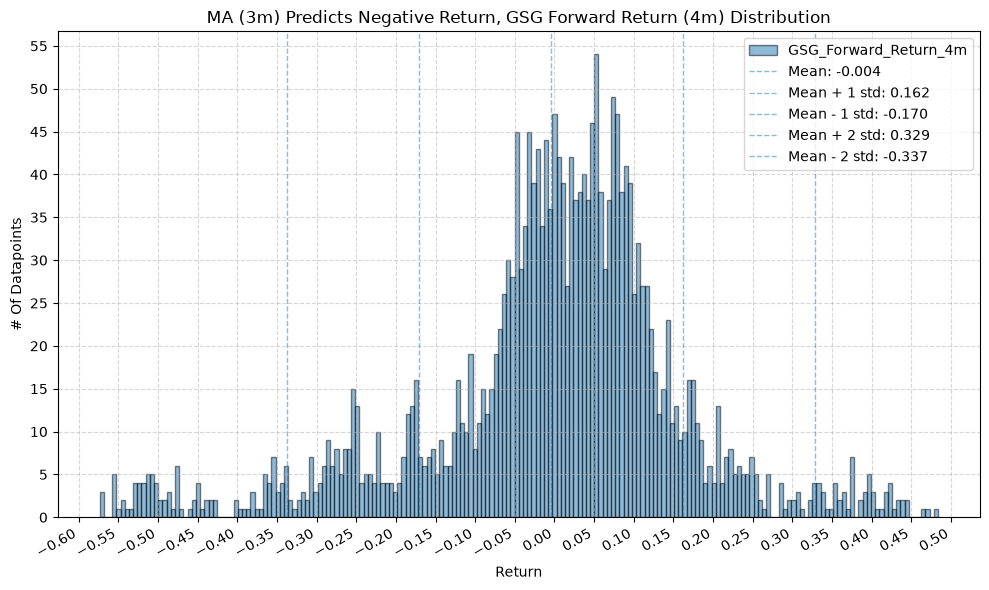
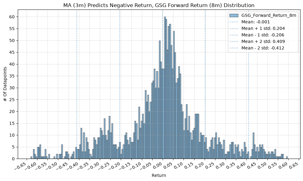
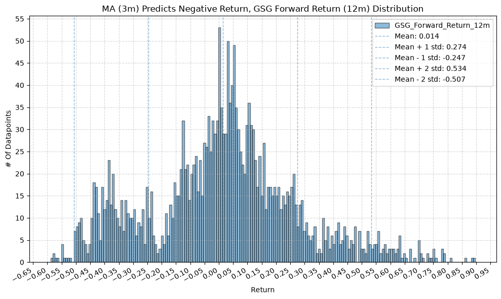
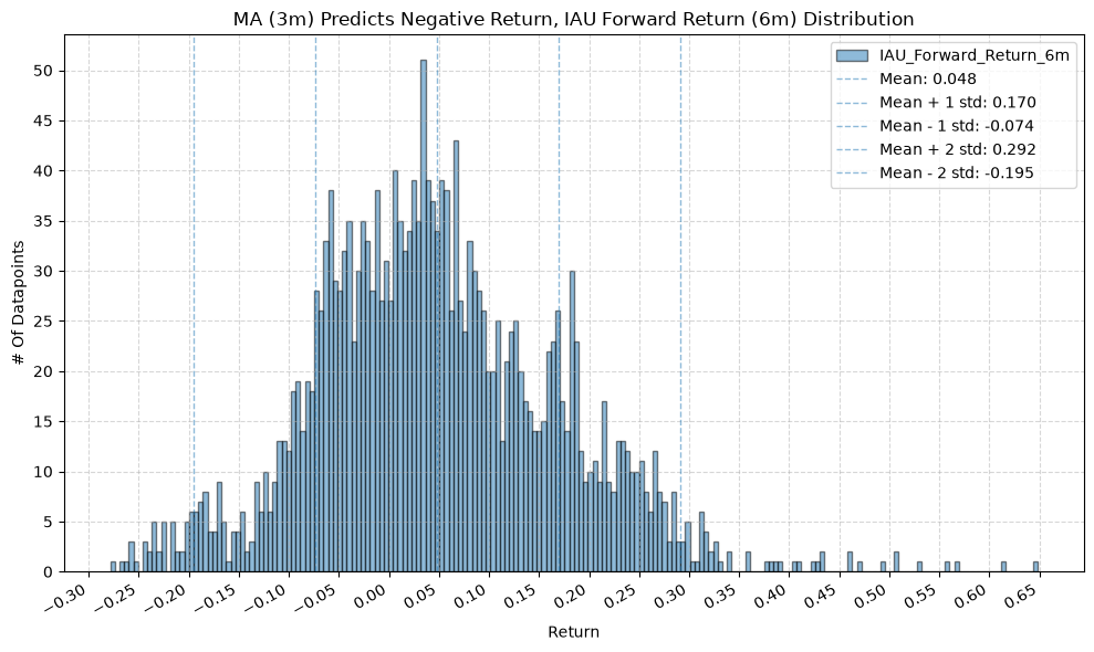
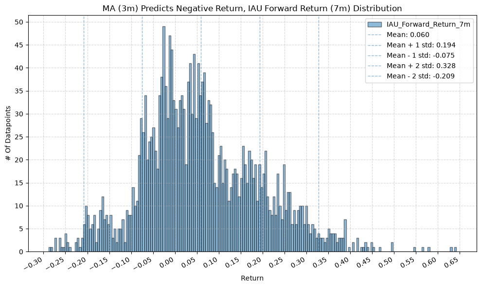
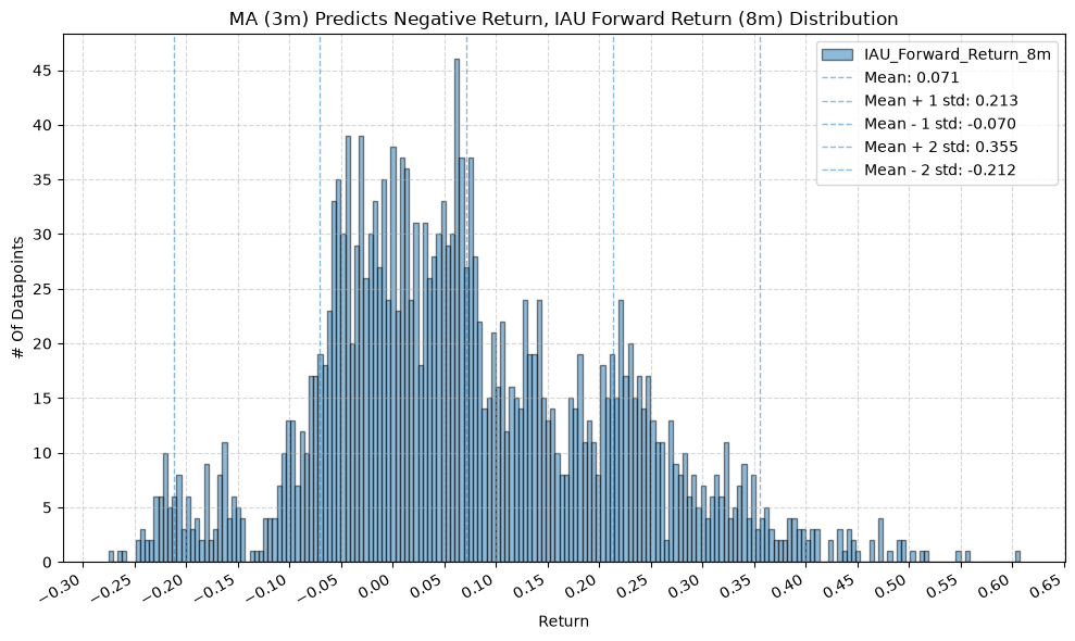
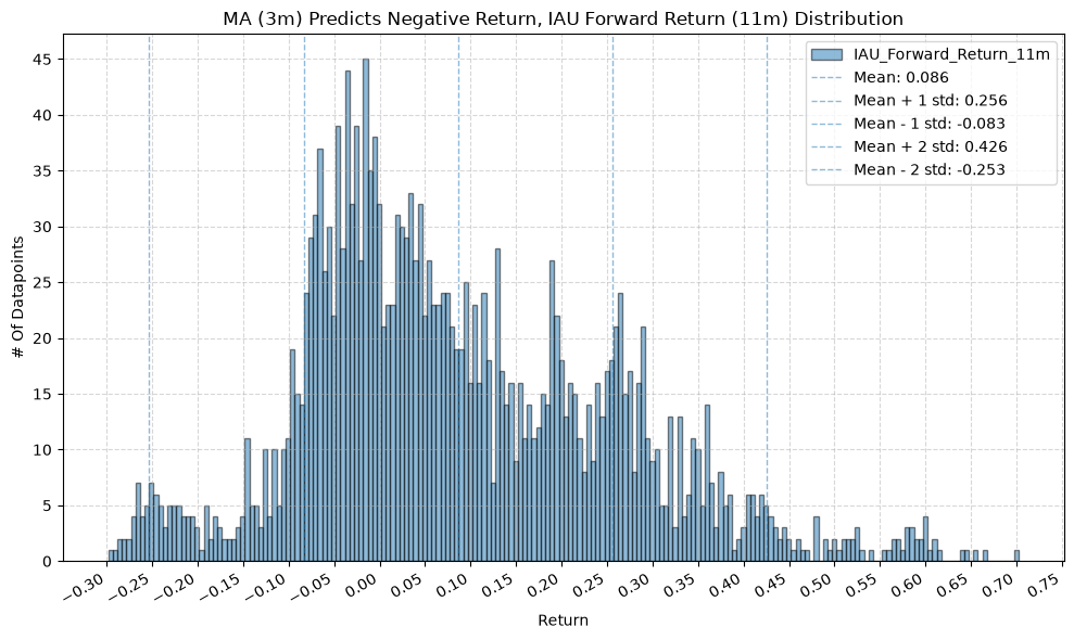
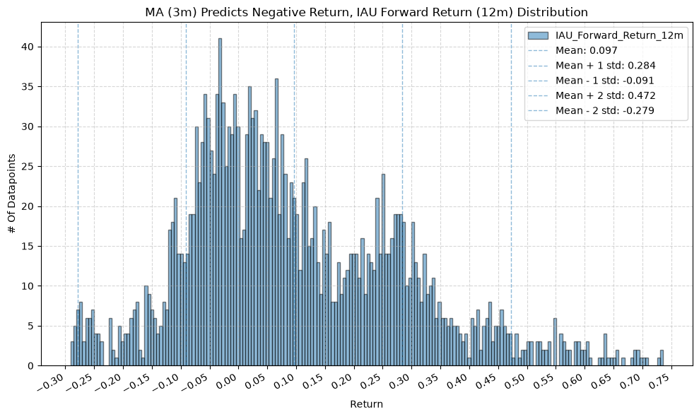
plot_histogram(
df=data[data[f"{fund}_MA_Prediction_{ma_label}"] == -1],
plot_columns=[f"{fund}_Forward_Return_{fr_label}"],
title=f"MA ({ma_label}) Predicts Negative Return, {fund} Forward Return ({fr_label}) Distribution",
x_label="Return",
x_tick_spacing="Auto",
x_tick_rotation=30,
y_label="# Of Datapoints",
y_tick_spacing="Auto",
y_tick_rotation=0,
grid=True,
legend=True,
export_plot=False,
plot_file_name=None,
)

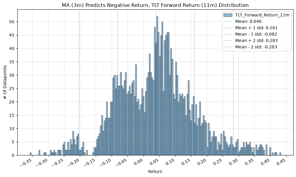
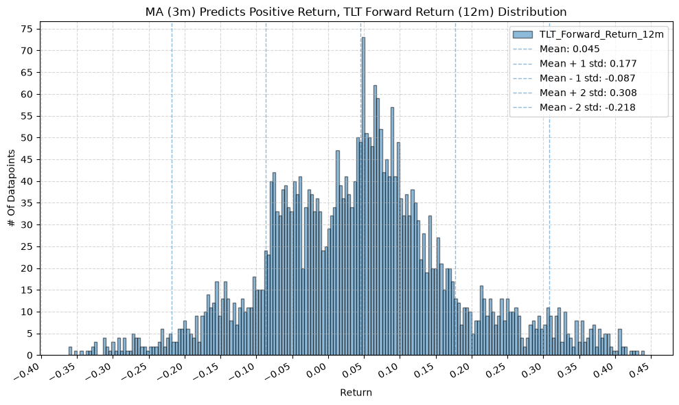
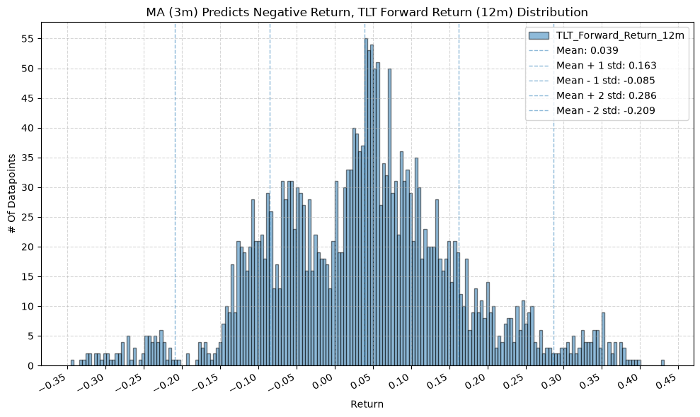
IEF and TLT #
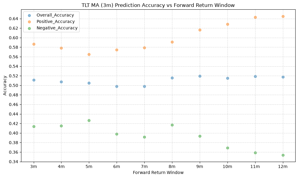
for fund, data in fund_data.items():
if fund not in ["IEF", "TLT"]:
continue
for ma_label, ma_window in ma_windows.items():
plot_scatter(
df=ma_prediction_results[(ma_prediction_results["Fund"] == fund) & (ma_prediction_results["MA_Window"] == ma_label)],
x_plot_column="Forward_Return_Window",
y_plot_columns=["Overall_Accuracy", "Positive_Accuracy", "Negative_Accuracy"],
title=f"{fund} MA ({ma_label}) Prediction Accuracy vs Forward Return Window",
x_label="Forward Return Window",
x_format="String",
x_format_decimal_places=0,
x_tick_spacing=1,
x_tick_start=None,
x_tick_rotation=0,
y_label="Accuracy",
y_format="Decimal",
y_format_decimal_places=2,
y_tick_spacing="Auto",
y_tick_rotation=0,
plot_OLS_regression_line=False,
OLS_column=None,
plot_Ridge_regression_line=False,
Ridge_column=None,
plot_RidgeCV_regression_line=False,
RidgeCV_column=None,
regression_constant=True,
grid=True,
legend=True,
export_plot=False,
plot_file_name=None,
)
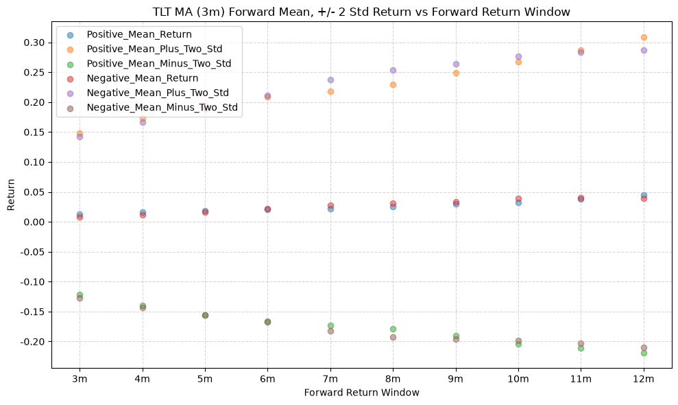
plot_scatter(
df=ma_prediction_results[(ma_prediction_results["Fund"] == fund) & (ma_prediction_results["MA_Window"] == ma_label)],
x_plot_column="Forward_Return_Window",
y_plot_columns=["Positive_Mean_Return", "Positive_Mean_Plus_Two_Std", "Positive_Mean_Minus_Two_Std", "Negative_Mean_Return", "Negative_Mean_Plus_Two_Std", "Negative_Mean_Minus_Two_Std"],
title=f"{fund} MA ({ma_label}) Forward Mean, +/- 2 Std Return vs Forward Return Window",
x_label="Forward Return Window",
x_format="String",
x_format_decimal_places=0,
x_tick_spacing=1,
x_tick_start=None,
x_tick_rotation=0,
y_label="Return",
y_format="Decimal",
y_format_decimal_places=2,
y_tick_spacing="Auto",
y_tick_rotation=0,
plot_OLS_regression_line=False,
OLS_column=None,
plot_Ridge_regression_line=False,
Ridge_column=None,
plot_RidgeCV_regression_line=False,
RidgeCV_column=None,
regression_constant=True,
grid=True,
legend=True,
export_plot=False,
plot_file_name=None,
)
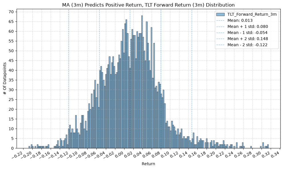
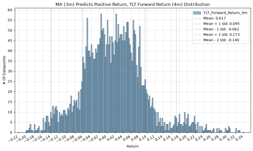
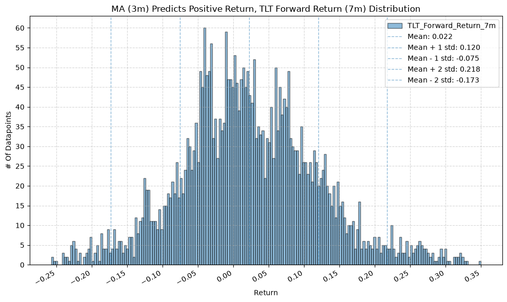
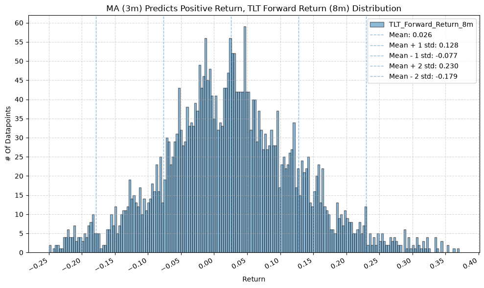
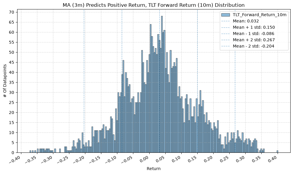
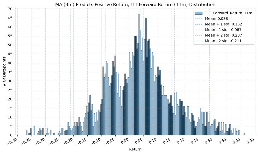
for fr_label, fr_window in forward_return_windows.items():
plot_histogram(
df=data[data[f"{fund}_MA_Prediction_{ma_label}"] == 1],
plot_columns=[f"{fund}_Forward_Return_{fr_label}"],
title=f"MA ({ma_label}) Predicts Positive Return, {fund} Forward Return ({fr_label}) Distribution",
x_label="Return",
x_tick_spacing="Auto",
x_tick_rotation=30,
y_label="# Of Datapoints",
y_tick_spacing="Auto",
y_tick_rotation=0,
grid=True,
legend=True,
export_plot=False,
plot_file_name=None,
)
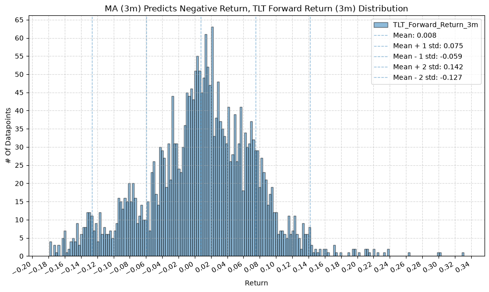
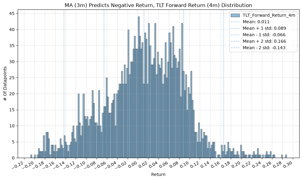
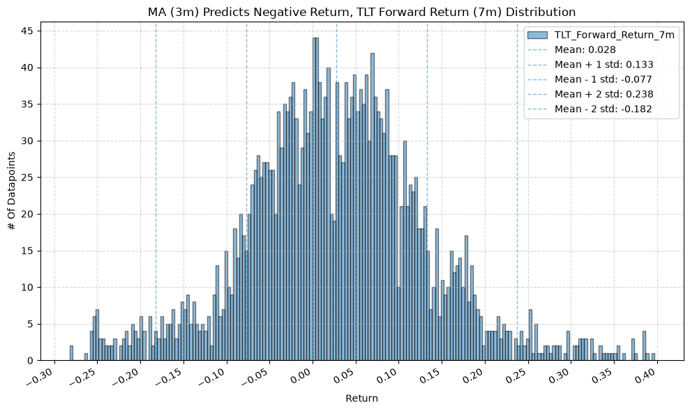
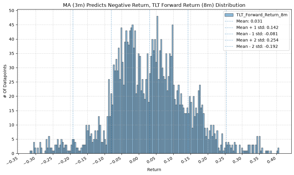
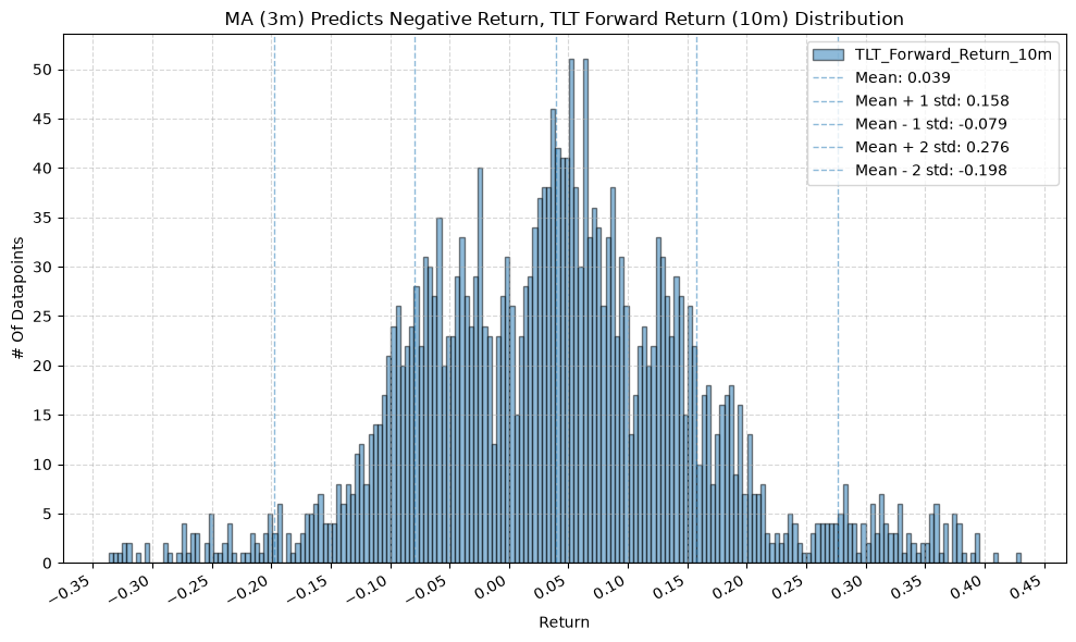
plot_histogram(
df=data[data[f"{fund}_MA_Prediction_{ma_label}"] == -1],
plot_columns=[f"{fund}_Forward_Return_{fr_label}"],
title=f"MA ({ma_label}) Predicts Negative Return, {fund} Forward Return ({fr_label}) Distribution",
x_label="Return",
x_tick_spacing="Auto",
x_tick_rotation=30,
y_label="# Of Datapoints",
y_tick_spacing="Auto",
y_tick_rotation=0,
grid=True,
legend=True,
export_plot=False,
plot_file_name=None,
)

# for fund, data in fund_data.items():
    # for ma_label, ma_window in ma_windows.items():
        # for fr_label, fr_window in forward_return_windows.items():
            # plot_scatter(
            #     df=data,
            #     x_plot_column=f"{fund}_Price_MA_Diff_Percent_{ma_label}",
            #     y_plot_columns=[f"{fund}_Forward_Return_{fr_label}"],
            #     title=f"{fund} MA Diff (Percent) ({ma_label}) vs Forward Return ({fr_label})",
            #     x_label="MA Diff (Percent)",
            #     x_format="Decimal",
            #     x_format_decimal_places=2,
            #     x_tick_spacing="Auto",
            #     x_tick_start=None,
            #     x_tick_rotation=30,
            #     y_label="Forward Return",
            #     y_format="Decimal",
            #     y_format_decimal_places=2,
            #     y_tick_spacing="Auto",
            #     y_tick_rotation=0,
            #     plot_OLS_regression_line=True,
            #     OLS_column=f"{fund}_Forward_Return_{fr_label}",
            #     plot_Ridge_regression_line=True,
            #     Ridge_column=f"{fund}_Forward_Return_{fr_label}",
            #     plot_RidgeCV_regression_line=True,
            #     RidgeCV_column=f"{fund}_Forward_Return_{fr_label}",
            #     regression_constant=True,
            #     grid=True,
            #     legend=True,
            #     export_plot=False,
            #     plot_file_name=None,
            # )
Analysis Of Results #
1. Positive, Negative, and Overall Accuracy #
From the above plots, we can see that some ETFs (which we are - kind of - using as a proxy for asset classes), appear to have a stronger relationship between the price-MA difference and the forward returns than others. This “relationship” takes the form of the overall accuracy of the predictions, which tells us how well the price-MA difference predicts the direction of the future returns.
1.1. Mean Overall Accuracy by Fund and MA Window #
Here we plot the overall mean prediction accuracy for each ETF and MA window combination.
# Calc overall mean accuracy for each fund across all MA windows
temp = ma_prediction_results.groupby(["Fund", "MA_Window"])["Overall_Accuracy"].mean().reset_index()

# Create a new DataFrame with unique MA_Window values and merge the mean accuracy for each fund
accuracy = pd.DataFrame({"MA_Window": temp["MA_Window"].unique()})

for fund in fund_list:
    fund_temp = temp[temp["Fund"] == fund][["MA_Window", "Overall_Accuracy"]].rename(
        columns={"Overall_Accuracy": f"{fund}_Overall_Accuracy"}
    )
    accuracy = pd.merge(accuracy, fund_temp, on="MA_Window", how="outer")

plot_scatter(
    df=accuracy,
    x_plot_column="MA_Window",
    y_plot_columns=["IVV_Overall_Accuracy",
                    "EFA_Overall_Accuracy",
                    "EEM_Overall_Accuracy",
                    "GSG_Overall_Accuracy",
                    "IAU_Overall_Accuracy",
                    "IEF_Overall_Accuracy",
                    "TLT_Overall_Accuracy"],
    title="Mean Overall Accuracy by Fund and MA Window",
    x_label="MA Window",
    x_format="String",
    x_format_decimal_places=0,
    x_tick_spacing=1,
    x_tick_start=None,
    x_tick_rotation=0,
    y_label="Accuracy",
    y_format="Decimal",
    y_format_decimal_places=2,
    y_tick_spacing="Auto",
    y_tick_rotation=0,
    plot_OLS_regression_line=False,
    OLS_column=None,
    plot_Ridge_regression_line=False,
    Ridge_column=None,
    plot_RidgeCV_regression_line=False,
    RidgeCV_column=None,
    regression_constant=True,
    grid=True,
    legend=True,
    legend_location="upper left",
    legend_anchor=(1, 1),
    export_plot=False,
    plot_file_name=None,
)
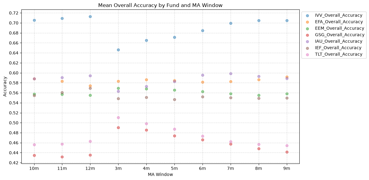
The stock funds (IVV, EFA, and EEM) have the highest mean overall accuracy, which tells us that the price-MA difference is a better predictor of the direction of future returns for these funds than for the other funds. The commodity fund (GSG) has the lowest mean overall accuracy, followed by long-term bonds (TLT), which both rank below the 50% threshold. If the mean overall accuracy does not exceed the 50% mark, then essentially the price-MA difference is not any better than a coin flip at predicting the direction of future returns.
1.2. Mean Positive Accuracy by Fund and MA Window #
The overall accuracy statistic includes the predicted accuracy of both the positive (are future returns positive when the price-MA is positive) and the negative (are future returns negative when the price-MA is negative) directions. The overall accuracy is useful from a long-short standpoint, but from a long-only perspective, we care only about the positive direction, which we plot next.
# Calc overall mean accuracy for each fund across all MA windows
temp = ma_prediction_results.groupby(["Fund", "MA_Window"])["Positive_Accuracy"].mean().reset_index()

for fund in fund_list:
    fund_temp = temp[temp["Fund"] == fund][["MA_Window", "Positive_Accuracy"]].rename(
        columns={"Positive_Accuracy": f"{fund}_Positive_Accuracy"}
    )
    accuracy = pd.merge(accuracy, fund_temp, on="MA_Window", how="outer")

plot_scatter(
    df=accuracy,
    x_plot_column="MA_Window",
    y_plot_columns=["IVV_Positive_Accuracy",
                    "EFA_Positive_Accuracy",
                    "EEM_Positive_Accuracy",
                    "GSG_Positive_Accuracy",
                    "IAU_Positive_Accuracy",
                    "IEF_Positive_Accuracy",
                    "TLT_Positive_Accuracy"],
    title="Mean Positive Accuracy by Fund and MA Window",
    x_label="MA Window",
    x_format="String",
    x_format_decimal_places=0,
    x_tick_spacing=1,
    x_tick_start=None,
    x_tick_rotation=0,
    y_label="Accuracy",
    y_format="Decimal",
    y_format_decimal_places=2,
    y_tick_spacing="Auto",
    y_tick_rotation=0,
    plot_OLS_regression_line=False,
    OLS_column=None,
    plot_Ridge_regression_line=False,
    Ridge_column=None,
    plot_RidgeCV_regression_line=False,
    RidgeCV_column=None,
    regression_constant=True,
    grid=True,
    legend=True,
    legend_location="upper left",
    legend_anchor=(1, 1),
    export_plot=False,
    plot_file_name=None,
)
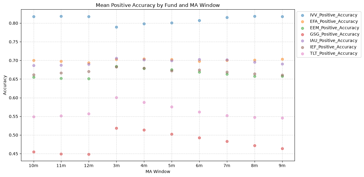
What we see is a nearly uniform shift up in the mean positive accuracy for all of the funds, relative to the overall accuracy. And not just by a little bit - it’s significant, as we will see below.
1.3. Difference Between Positive and Overall Accuracy by Fund and MA Window #
Here’s the plot of the difference betweent he mean and positive accuracy.
for fund in fund_list:
    accuracy[f"{fund}_Positive_Overall_Mean_Diff"] = accuracy[f"{fund}_Positive_Accuracy"] - accuracy[f"{fund}_Overall_Accuracy"]

plot_scatter(
    df=accuracy,
    x_plot_column="MA_Window",
    y_plot_columns=["IVV_Positive_Overall_Mean_Diff",
                    "EFA_Positive_Overall_Mean_Diff",
                    "EEM_Positive_Overall_Mean_Diff",
                    "GSG_Positive_Overall_Mean_Diff",
                    "IAU_Positive_Overall_Mean_Diff",
                    "IEF_Positive_Overall_Mean_Diff",
                    "TLT_Positive_Overall_Mean_Diff"],
    title="Difference Between Positive and Overall Accuracy by Fund and MA Window",
    x_label="MA Window",
    x_format="String",
    x_format_decimal_places=0,
    x_tick_spacing=1,
    x_tick_start=None,
    x_tick_rotation=0,
    y_label="Accuracy Difference",
    y_format="Decimal",
    y_format_decimal_places=2,
    y_tick_spacing="Auto",
    y_tick_rotation=0,
    plot_OLS_regression_line=False,
    OLS_column=None,
    plot_Ridge_regression_line=False,
    Ridge_column=None,
    plot_RidgeCV_regression_line=False,
    RidgeCV_column=None,
    regression_constant=True,
    grid=True,
    legend=True,
    legend_location="upper left",
    legend_anchor=(1, 1),
    export_plot=False,
    plot_file_name=None,
)
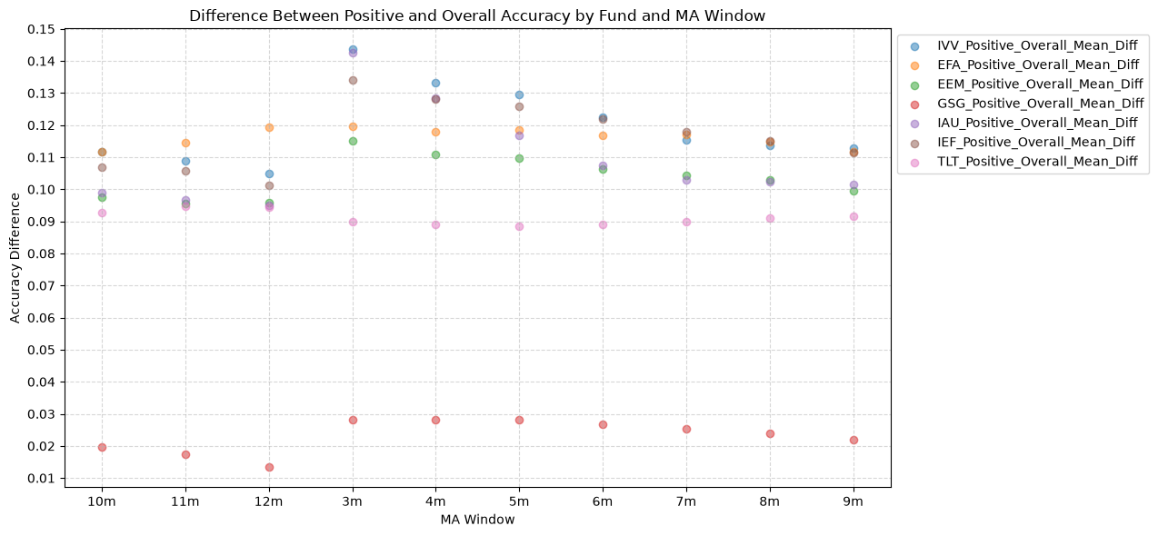
IVV shows a 10 - 14% difference, while GSG show only a 2 or 3% improvement. The other funds show a 9 - 12%. If we were interested in using the price-MA difference to predict the direction of future returns, we would be better off using only the positive predictions.
2. Distribution of Future Returns Based on Price-MA Difference #
Next, we can consider the shape of the distribution of the future returns, split on whether the the price-MA difference is positive or negative.
2.1. Mean Future Return When Price-MA Difference is Positive by Fund and MA Window #
First, the distribution of future returns when the price-MA difference is positive.
temp = ma_prediction_results.groupby(["Fund", "MA_Window"])["Positive_Mean_Return"].mean().reset_index()

distribution = pd.DataFrame({"MA_Window": temp["MA_Window"].unique()})

for fund in fund_list:
    fund_temp = temp[temp["Fund"] == fund][["MA_Window", "Positive_Mean_Return"]].rename(
        columns={"Positive_Mean_Return": f"{fund}_Positive_Mean_Return"}
    )
    distribution = pd.merge(distribution, fund_temp, on="MA_Window", how="outer")

plot_scatter(
    df=distribution,
    x_plot_column="MA_Window",
    y_plot_columns=["IVV_Positive_Mean_Return",
                    "EFA_Positive_Mean_Return",
                    "EEM_Positive_Mean_Return",
                    "GSG_Positive_Mean_Return",
                    "IAU_Positive_Mean_Return",
                    "IEF_Positive_Mean_Return",
                    "TLT_Positive_Mean_Return"],
    title="Mean Future Return When Price-MA Difference is Positive by Fund and MA Window",
    x_label="MA Window",
    x_format="String",
    x_format_decimal_places=0,
    x_tick_spacing=1,
    x_tick_start=None,
    x_tick_rotation=0,
    y_label="Return",
    y_format="Decimal",
    y_format_decimal_places=3,
    y_tick_spacing="Auto",
    y_tick_rotation=0,
    plot_OLS_regression_line=False,
    OLS_column=None,
    plot_Ridge_regression_line=False,
    Ridge_column=None,
    plot_RidgeCV_regression_line=False,
    RidgeCV_column=None,
    regression_constant=True,
    grid=True,
    legend=True,
    legend_location="upper left",
    legend_anchor=(1, 1),
    export_plot=False,
    plot_file_name=None,
)
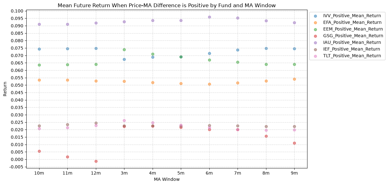
In a perfect world, we want to see similar numbers across all MA windows, and all of those numbers would be relatively high. If every window gives us roughly the same distribution of future returns, that would indicate a consistent predictive relationship across all windows. But, what we often see is that the distributions vary quite a bit depending on the window, which suggests that it’s useful to consider a combination of windows to form a more robust signal.
Note that gold (IAU) has a smaller variation and much higher values (mean return is ~1.5% greater than IVV) across MA windows compared to the other funds.
2.2. Mean Future Return When Price-MA Difference is Negative by Fund and MA Window #
On to the distribution of future returns when the price-MA difference is negative.
temp = ma_prediction_results.groupby(["Fund", "MA_Window"])["Negative_Mean_Return"].mean().reset_index()

for fund in fund_list:
    fund_temp = temp[temp["Fund"] == fund][["MA_Window", "Negative_Mean_Return"]].rename(
        columns={"Negative_Mean_Return": f"{fund}_Negative_Mean_Return"}
    )
    distribution = pd.merge(distribution, fund_temp, on="MA_Window", how="outer")

plot_scatter(
    df=distribution,
    x_plot_column="MA_Window",
    y_plot_columns=["IVV_Negative_Mean_Return",
                    "EFA_Negative_Mean_Return",
                    "EEM_Negative_Mean_Return",
                    "GSG_Negative_Mean_Return",
                    "IAU_Negative_Mean_Return",
                    "IEF_Negative_Mean_Return",
                    "TLT_Negative_Mean_Return"],
    title="Mean Future Return When Price-MA Difference is Negative by Fund and MA Window",
    x_label="MA Window",
    x_format="String",
    x_format_decimal_places=0,
    x_tick_spacing=1,
    x_tick_start=None,
    x_tick_rotation=0,
    y_label="Return",
    y_format="Decimal",
    y_format_decimal_places=3,
    y_tick_spacing="Auto",
    y_tick_rotation=0,
    plot_OLS_regression_line=False,
    OLS_column=None,
    plot_Ridge_regression_line=False,
    Ridge_column=None,
    plot_RidgeCV_regression_line=False,
    RidgeCV_column=None,
    regression_constant=True,
    grid=True,
    legend=True,
    legend_location="upper left",
    legend_anchor=(1, 1),
    export_plot=False,
    plot_file_name=None,
)
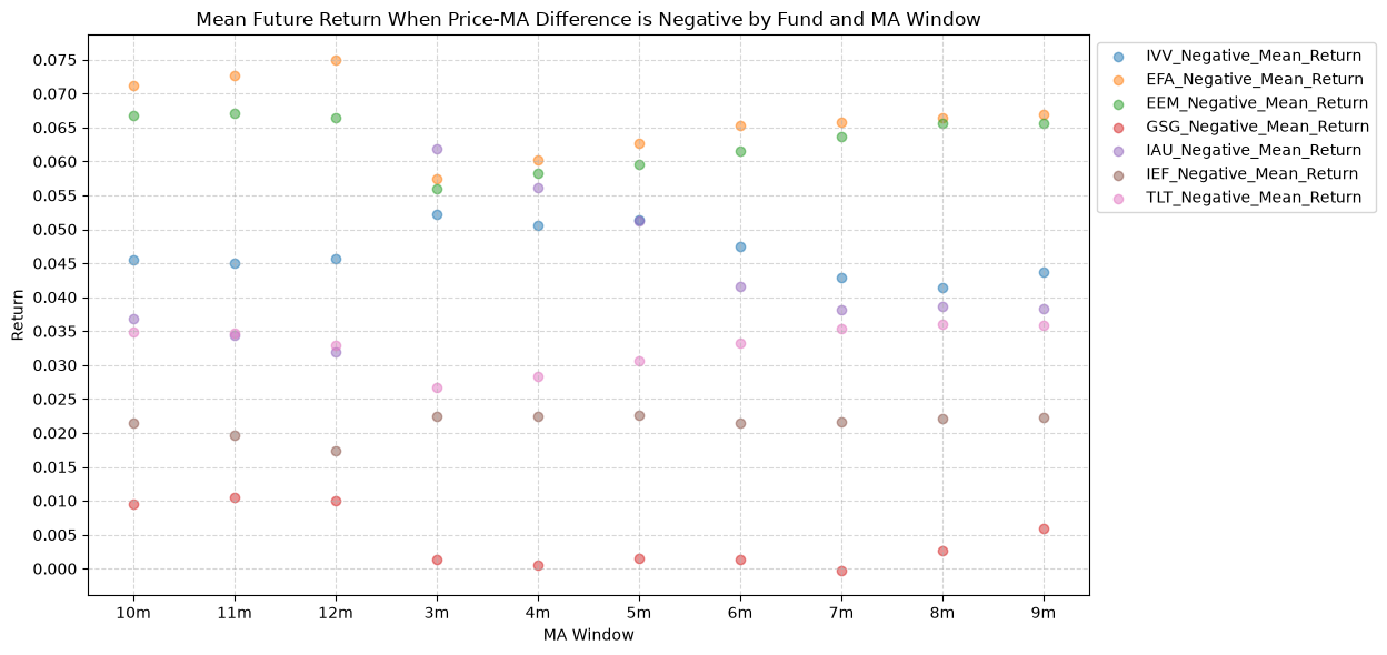
Interesting, the mean returns are mostly still positive. That suggests that even when the price-MA difference is negative, future returns tend to be positive on average, though perhaps smaller than when the difference is positive.
2.3. Difference Between Predicted Positive and Negative Mean Returns by Fund and MA Window #
Next, we can look at the difference in mean future returns between when the price-MA difference is positive and when it is negative.
for fund in fund_list:
    distribution[f"{fund}_Mean_Return_Diff"] = distribution[f"{fund}_Positive_Mean_Return"] - distribution[f"{fund}_Negative_Mean_Return"]

plot_scatter(
    df=distribution,
    x_plot_column="MA_Window",
    y_plot_columns=["IVV_Mean_Return_Diff",
                    "EFA_Mean_Return_Diff",
                    "EEM_Mean_Return_Diff",
                    "GSG_Mean_Return_Diff",
                    "IAU_Mean_Return_Diff",
                    "IEF_Mean_Return_Diff",
                    "TLT_Mean_Return_Diff"],
    title="Difference Between Predicted Positive and Negative Mean Returns by Fund and MA Window",
    x_label="MA Window",
    x_format="String",
    x_format_decimal_places=0,
    x_tick_spacing=1,
    x_tick_start=None,
    x_tick_rotation=0,
    y_label="Return Difference",
    y_format="Decimal",
    y_format_decimal_places=2,
    y_tick_spacing="Auto",
    y_tick_rotation=0,
    plot_OLS_regression_line=False,
    OLS_column=None,
    plot_Ridge_regression_line=False,
    Ridge_column=None,
    plot_RidgeCV_regression_line=False,
    RidgeCV_column=None,
    regression_constant=True,
    grid=True,
    legend=True,
    legend_location="upper left",
    legend_anchor=(1, 1),
    export_plot=False,
    plot_file_name=None,
)
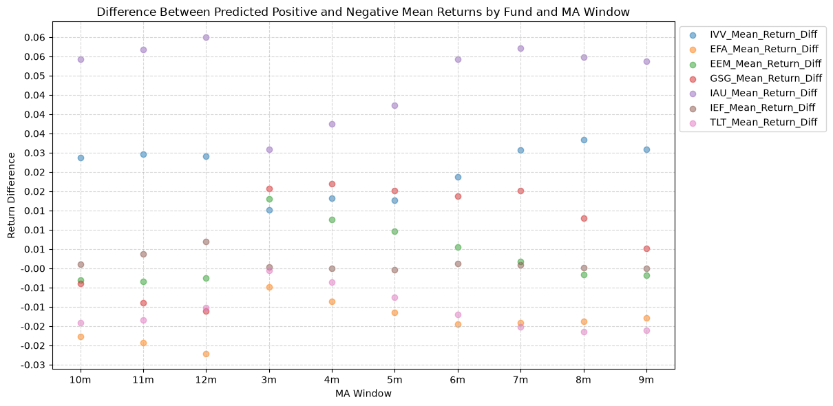
In general, the mean of the future positive predicted returns is higher than the mean of the future negative predicted returns, which is what we would expect if the price-MA difference has any predictive power. However, the distributions are not normal, and there are some outliers that skew the distributions. These outliers show up as the long tails in the distributions, and the number and magnitude of the outliers can be seen in the mean +/- 2 standard deviations.
Note again, gold has the highest difference in mean return between when the price-MA difference is positive and when it is negative.
2.4. Difference Between Positive Mean +2 Std and Positive Mean -2 Std Returns by Fund and MA Window #
As mentioned above, we think that there are outliers that skew the distributions of the forward returns. But by how much? And how can we quantify their impact? One way is to look at the standard deviations. Here’s the plots for the difference between 2 standard deviations above and below the mean for the forward returns.
temp = ma_prediction_results.groupby(["Fund", "MA_Window"])["Positive_Mean_Plus_Two_Std"].mean().reset_index()

for fund in fund_list:
    fund_temp = temp[temp["Fund"] == fund][["MA_Window", "Positive_Mean_Plus_Two_Std"]].rename(
        columns={"Positive_Mean_Plus_Two_Std": f"{fund}_Positive_Mean_Plus_Two_Std"}
    )
    distribution = pd.merge(distribution, fund_temp, on="MA_Window", how="outer")

temp = ma_prediction_results.groupby(["Fund", "MA_Window"])["Positive_Mean_Minus_Two_Std"].mean().reset_index()

for fund in fund_list:
    fund_temp = temp[temp["Fund"] == fund][["MA_Window", "Positive_Mean_Minus_Two_Std"]].rename(
        columns={"Positive_Mean_Minus_Two_Std": f"{fund}_Positive_Mean_Minus_Two_Std"}
    )
    distribution = pd.merge(distribution, fund_temp, on="MA_Window", how="outer")

for fund in fund_list:
    distribution[f"{fund}_Positive_Mean_Plus_Minus_2Std_Diff"] = distribution[f"{fund}_Positive_Mean_Plus_Two_Std"] - distribution[f"{fund}_Positive_Mean_Minus_Two_Std"]

plot_scatter(
    df=distribution,
    x_plot_column="MA_Window",
    y_plot_columns=["IVV_Positive_Mean_Plus_Minus_2Std_Diff",
                    "EFA_Positive_Mean_Plus_Minus_2Std_Diff",
                    "EEM_Positive_Mean_Plus_Minus_2Std_Diff",
                    "GSG_Positive_Mean_Plus_Minus_2Std_Diff",
                    "IAU_Positive_Mean_Plus_Minus_2Std_Diff",
                    "IEF_Positive_Mean_Plus_Minus_2Std_Diff",
                    "TLT_Positive_Mean_Plus_Minus_2Std_Diff"],
    title="Difference Between Positive Mean +2 Std and Positive Mean -2 Std Returns by Fund and MA Window",
    x_label="MA Window",
    x_format="String",
    x_format_decimal_places=0,
    x_tick_spacing=1,
    x_tick_start=None,
    x_tick_rotation=0,
    y_label="Mean Return 2 Std Difference",
    y_format="Decimal",
    y_format_decimal_places=3,
    y_tick_spacing="Auto",
    y_tick_rotation=0,
    plot_OLS_regression_line=False,
    OLS_column=None,
    plot_Ridge_regression_line=False,
    Ridge_column=None,
    plot_RidgeCV_regression_line=False,
    RidgeCV_column=None,
    regression_constant=True,
    grid=True,
    legend=True,
    legend_location="upper left",
    legend_anchor=(1, 1),
    export_plot=False,
    plot_file_name=None,
)
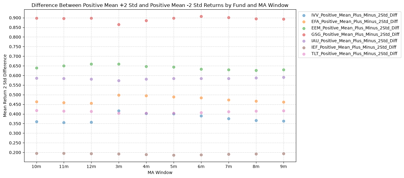
GSG is a mess… the commodity fund has a lot of noise and outliers. We’d like to see a tight distribution, that might give us confidence that the forward returns are within a reasonable range and not being dominated by extreme values. Here, the 7-10 year bond ETF is the leader, with a much tighter distribution and fewer extreme values skewing the results.
2.5. Difference Between Negative Mean +2 Std and Negative Mean -2 Std Returns by Fund and MA Window #
Now for the e difference between 2 standard deviations above and below the mean for the forward returns when price-MA is negative.
temp = ma_prediction_results.groupby(["Fund", "MA_Window"])["Negative_Mean_Plus_Two_Std"].mean().reset_index()

for fund in fund_list:
    fund_temp = temp[temp["Fund"] == fund][["MA_Window", "Negative_Mean_Plus_Two_Std"]].rename(
        columns={"Negative_Mean_Plus_Two_Std": f"{fund}_Negative_Mean_Plus_Two_Std"}
    )
    distribution = pd.merge(distribution, fund_temp, on="MA_Window", how="outer")

temp = ma_prediction_results.groupby(["Fund", "MA_Window"])["Negative_Mean_Minus_Two_Std"].mean().reset_index()

for fund in fund_list:
    fund_temp = temp[temp["Fund"] == fund][["MA_Window", "Negative_Mean_Minus_Two_Std"]].rename(
        columns={"Negative_Mean_Minus_Two_Std": f"{fund}_Negative_Mean_Minus_Two_Std"}
    )
    distribution = pd.merge(distribution, fund_temp, on="MA_Window", how="outer")

for fund in fund_list:
    distribution[f"{fund}_Negative_Mean_Plus_Minus_2Std_Diff"] = distribution[f"{fund}_Negative_Mean_Plus_Two_Std"] - distribution[f"{fund}_Negative_Mean_Minus_Two_Std"]

plot_scatter(
    df=distribution,
    x_plot_column="MA_Window",
    y_plot_columns=["IVV_Negative_Mean_Plus_Minus_2Std_Diff",
                    "EFA_Negative_Mean_Plus_Minus_2Std_Diff",
                    "EEM_Negative_Mean_Plus_Minus_2Std_Diff",
                    "GSG_Negative_Mean_Plus_Minus_2Std_Diff",
                    "IAU_Negative_Mean_Plus_Minus_2Std_Diff",
                    "IEF_Negative_Mean_Plus_Minus_2Std_Diff",
                    "TLT_Negative_Mean_Plus_Minus_2Std_Diff"],
    title="Difference Between Negative Mean +2 Std and Negative Mean -2 Std Returns by Fund and MA Window",
    x_label="MA Window",
    x_format="String",
    x_format_decimal_places=0,
    x_tick_spacing=1,
    x_tick_start=None,
    x_tick_rotation=0,
    y_label="Mean Return 2 Std Difference",
    y_format="Decimal",
    y_format_decimal_places=3,
    y_tick_spacing="Auto",
    y_tick_rotation=0,
    plot_OLS_regression_line=False,
    OLS_column=None,
    plot_Ridge_regression_line=False,
    Ridge_column=None,
    plot_RidgeCV_regression_line=False,
    RidgeCV_column=None,
    regression_constant=True,
    grid=True,
    legend=True,
    legend_location="upper left",
    legend_anchor=(1, 1),
    export_plot=False,
    plot_file_name=None,
)
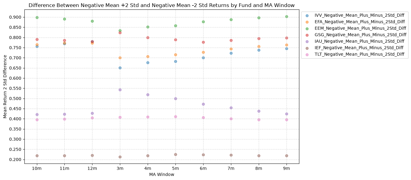
This might not be as relevant to us (from a long-only perspective), but it’s still worth looking at to understand how the asset classes rank. Emerging markets tend to have more volatility and outliers, so this plot makes sense intuitively.
2.6. Difference Between Positive and Negative +/-2 Std Return Spreads by Fund and MA Window #
Finally, we have the difference between the 2 standard deviation spreads.
for fund in fund_list:
    distribution[f"{fund}_2Std_Spread_Diff"] = distribution[f"{fund}_Positive_Mean_Plus_Minus_2Std_Diff"] - distribution[f"{fund}_Negative_Mean_Plus_Minus_2Std_Diff"]

plot_scatter(
    df=distribution,
    x_plot_column="MA_Window",
    y_plot_columns=["IVV_2Std_Spread_Diff",
                    "EFA_2Std_Spread_Diff",
                    "EEM_2Std_Spread_Diff",
                    "GSG_2Std_Spread_Diff",
                    "IAU_2Std_Spread_Diff",
                    "IEF_2Std_Spread_Diff",
                    "TLT_2Std_Spread_Diff"],
    title="Difference Between Positive and Negative +/-2 Std Return Spreads by Fund and MA Window",
    x_label="MA Window",
    x_format="String",
    x_format_decimal_places=0,
    x_tick_spacing=1,
    x_tick_start=None,
    x_tick_rotation=0,
    y_label="Mean Return 2 Std Difference (Positive - Negative)",
    y_format="Decimal",
    y_format_decimal_places=3,
    y_tick_spacing="Auto",
    y_tick_rotation=0,
    plot_OLS_regression_line=False,
    OLS_column=None,
    plot_Ridge_regression_line=False,
    Ridge_column=None,
    plot_RidgeCV_regression_line=False,
    RidgeCV_column=None,
    regression_constant=True,
    grid=True,
    legend=True,
    legend_location="upper left",
    legend_anchor=(1, 1),
    export_plot=False,
    plot_file_name=None,
)
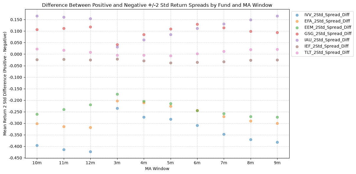
This plot really compares the kurtosis of the forward return distributions by looking at the difference between the 2 standard deviation spreads for positive and negative price-MA conditions. If these values are positive, it means that the forward return distributions have fatter tails for positive price-MA conditions relative to negative price-MA conditions, and the opposite is true if the values are negative.
So anything <=0 is good here, which brings us back to gold, which is positive. Pulling up one of the earlier plots:
for fund, data in fund_data.items():
    if fund not in ["IAU"]:
        continue
    for ma_label, ma_window in ma_windows.items():
        plot_scatter(
            df=ma_prediction_results[(ma_prediction_results["Fund"] == fund) & (ma_prediction_results["MA_Window"] == ma_label)],
            x_plot_column="Forward_Return_Window",
            y_plot_columns=["Positive_Mean_Return", "Positive_Mean_Plus_Two_Std", "Positive_Mean_Minus_Two_Std", "Negative_Mean_Return", "Negative_Mean_Plus_Two_Std", "Negative_Mean_Minus_Two_Std"],
            title=f"{fund} MA ({ma_label}) Forward Mean, +/- 2 Std Return vs Forward Return Window",
            x_label="Forward Return Window",
            x_format="String",
            x_format_decimal_places=0,
            x_tick_spacing=1,
            x_tick_start=None,
            x_tick_rotation=0,
            y_label="Return",
            y_format="Decimal",
            y_format_decimal_places=2,
            y_tick_spacing="Auto",
            y_tick_rotation=0,
            plot_OLS_regression_line=False,
            OLS_column=None,
            plot_Ridge_regression_line=False,
            Ridge_column=None,
            plot_RidgeCV_regression_line=False,
            RidgeCV_column=None,
            regression_constant=True,
            grid=True,
            legend=True,
            export_plot=False,
            plot_file_name=None,
        )
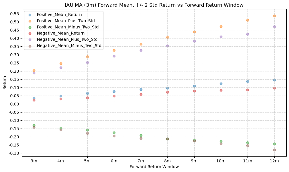
We can see that the mean +2 std return line is for the positive price-MA condition is actually above the mean +2 std return line for the negative price-MA condition, whichi is different than any of the other funds. The explanation? The forward positive return tail is fatter, which is actually a more desirable condition. While we’d like a tight distribution, we also will accept a fatter positive tail, as that means that the forward returns are more likely to be positive and larger than they would be otherwise.
Conclusion #
This analysis shows that the predictive power of moving averages varies across different asset classes. While some ETFs, particularly those representing equities, demonstrate a stronger relationship between price-MA differences and future returns, others, like commodities and long-term bonds, show less predictive power. The findings suggest that investors may benefit from using the price-MA relationship when developing trend following investment strategies.
Code #
The Jupyter notebook with the functions and all other code is available here.The HTML export of the jupyter notebook is available here.
The PDF export of the jupyter notebook is available here.