Leveraged ETF Return Dispersion

Table of Contents
Introduction #
Over the past 15 years (or so), leveraged ETFs have become frequently used for trading equity indices, sectors, and other asset classes by the investor that is seeking to use leverage for excess exposure to those asset classes. The question remains, however, what happens to the returns of leveraged ETFs over an extended time horizon and is there an optimal leverage ratio for the long-term buy-and-hold investor that allows them to take advantage of leverage to increase the up-side returns, while avoiding catastrophic losses on the down-side? In this investigation, we will delve into these ideas and see what the data shows.
Python Imports #
# Standard Library
import os
import sys
import warnings

from pathlib import Path

# Data Handling
import pandas as pd

# Suppress warnings
warnings.filterwarnings("ignore")
# Add the source subdirectory to the system path to allow import config from settings.py
current_directory = Path(os.getcwd())
website_base_directory = current_directory.parent.parent.parent
src_directory = website_base_directory / "src"
sys.path.append(str(src_directory)) if str(src_directory) not in sys.path else None

# Import settings.py
from settings import config

# Add configured directories from config to path
SOURCE_DIR = config("SOURCE_DIR")
sys.path.append(str(Path(SOURCE_DIR))) if str(Path(SOURCE_DIR)) not in sys.path else None

# Add other configured directories
BASE_DIR = config("BASE_DIR")
CONTENT_DIR = config("CONTENT_DIR")
POSTS_DIR = config("POSTS_DIR")
PAGES_DIR = config("PAGES_DIR")
PUBLIC_DIR = config("PUBLIC_DIR")
SOURCE_DIR = config("SOURCE_DIR")
DATA_DIR = config("DATA_DIR")
DATA_MANUAL_DIR = config("DATA_MANUAL_DIR")
Python Functions #
Here are the functions needed for this project:
- load_data: Load data from a CSV, Excel, or Pickle file into a pandas DataFrame.
- pandas_set_decimal_places: Set the number of decimal places displayed for floating-point numbers in pandas.
- plot_histogram: Plot the histogram of a data set from a DataFrame.
- plot_scatter: Plot the data from a DataFrame for a specified date range and columns.
- plot_time_series: Plot the timeseries data from a DataFrame for a specified date range and columns.
- run_linear_regression: Run a linear regression using statsmodels OLS and return the results.
- summary_stats: Generate summary statistics for a series of returns.
- yf_pull_data: Download daily price data from Yahoo Finance and export it.
from load_data import load_data
from pandas_set_decimal_places import pandas_set_decimal_places
from plot_histogram import plot_histogram
from plot_scatter import plot_scatter
from plot_time_series import plot_time_series
from run_linear_regression import run_linear_regression
from summary_stats import summary_stats
from yf_pull_data import yf_pull_data
Data Overview #
For this exercise, we will investigate the long-term return relationships between the following:
- QQQ (Invesco QQQ Trust, Series 1) and TQQQ (ProShares UltraPro QQQ)
- SPY (SPDR S&P 500 ETF Trust) and UPRO (ProShares UltraPro S&P 500)
Just to clarify, any time we are referring to “close prices” in this analysis, we are referring to the partially-adjusted close prices that account for splits, but not dividends. Because we are dealing with leveraged ETFs, we want to focus on the pure returns due to change in price, but exclude the dividends, which are not leveraged in the same way as the price changes.
QQQ & TQQQ #
Acquire & Plot Data (QQQ) #
First, let’s get the data for QQQ. If we already have the desired data, we can load it from a local pickle file. Otherwise, we can download it from Yahoo Finance using the yf_pull_data function.
pandas_set_decimal_places(2)

yf_pull_data(
    base_directory=DATA_DIR,
    ticker="QQQ",
    adjusted=False,
    source="Yahoo_Finance",
    asset_class="Exchange_Traded_Funds",
    excel_export=True,
    pickle_export=True,
    output_confirmation=False,
)

qqq = load_data(
    base_directory=DATA_DIR,
    ticker="QQQ",
    source="Yahoo_Finance",
    asset_class="Exchange_Traded_Funds",
    timeframe="Daily",
    file_format="pickle",
)

# Rename columns to "QQQ_Close", etc.
qqq = qqq.rename(columns={
    "Adj Close": "QQQ_Adj_Close",
    "Close": "QQQ_Close",
    "High": "QQQ_High",
    "Low": "QQQ_Low",
    "Open": "QQQ_Open",
    "Volume": "QQQ_Volume"
})

display(qqq)
| QQQ_Adj_Close | QQQ_Close | QQQ_High | QQQ_Low | QQQ_Open | QQQ_Volume | |
|---|---|---|---|---|---|---|
| Date | ||||||
| 1999-03-10 | 43.13 | 51.06 | 51.16 | 50.28 | 51.12 | 5232000 |
| 1999-03-11 | 43.34 | 51.31 | 51.73 | 50.31 | 51.44 | 9688600 |
| 1999-03-12 | 42.28 | 50.06 | 51.16 | 49.66 | 51.12 | 8743600 |
| 1999-03-15 | 43.50 | 51.50 | 51.56 | 49.91 | 50.44 | 6369000 |
| 1999-03-16 | 43.87 | 51.94 | 52.16 | 51.16 | 51.72 | 4905800 |
| ... | ... | ... | ... | ... | ... | ... |
| 2026-03-16 | 600.38 | 600.38 | 603.86 | 599.11 | 600.04 | 49077200 |
| 2026-03-17 | 603.31 | 603.31 | 605.90 | 601.87 | 603.14 | 47106600 |
| 2026-03-18 | 594.90 | 594.90 | 603.16 | 594.56 | 601.49 | 56128000 |
| 2026-03-19 | 593.02 | 593.02 | 595.80 | 587.08 | 589.51 | 75597600 |
| 2026-03-20 | 582.06 | 582.06 | 591.17 | 578.54 | 591.06 | 91964700 |
6800 rows × 6 columns
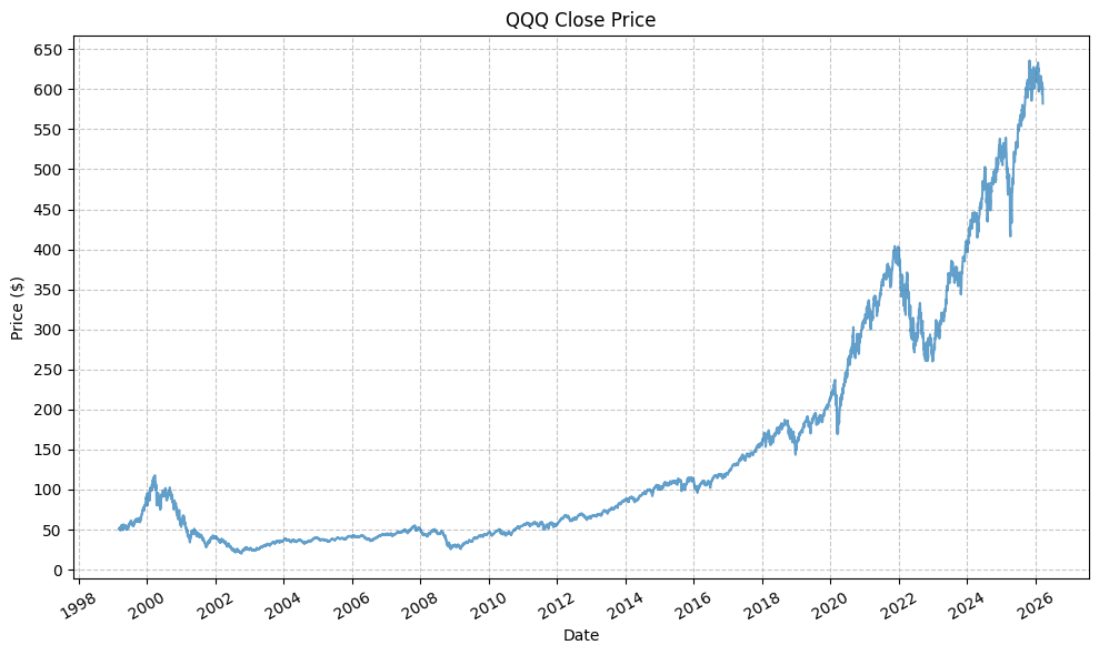
And the plot of the time series of partially adjusted close prices:
plot_time_series(
    df=qqq,
    plot_start_date=None,
    plot_end_date=None,
    plot_columns=["QQQ_Close"],
    title="QQQ Close Price",
    x_label="Date",
    x_format="Year",
    x_tick_spacing=2,
    x_tick_rotation=30,
    y_label="Price ($)",
    y_format="Decimal",
    y_format_decimal_places=0,
    y_tick_spacing="Auto",
    y_tick_rotation=0,
    grid=True,
    legend=False,
    export_plot=False,
    plot_file_name=None,
)
Acquire & Plot Data (TQQQ) #
Next, TQQQ:
yf_pull_data(
    base_directory=DATA_DIR,
    ticker="TQQQ",
    adjusted=False,
    source="Yahoo_Finance",
    asset_class="Exchange_Traded_Funds",
    excel_export=True,
    pickle_export=True,
    output_confirmation=False,
)

tqqq = load_data(
    base_directory=DATA_DIR,
    ticker="TQQQ",
    source="Yahoo_Finance",
    asset_class="Exchange_Traded_Funds",
    timeframe="Daily",
    file_format="pickle",
)

# Rename columns to "TQQQ_Close", etc.
tqqq = tqqq.rename(columns={
    "Adj Close": "TQQQ_Adj_Close",
    "Close": "TQQQ_Close",
    "High": "TQQQ_High",
    "Low": "TQQQ_Low",
    "Open": "TQQQ_Open",
    "Volume": "TQQQ_Volume"
})

display(tqqq)
| TQQQ_Adj_Close | TQQQ_Close | TQQQ_High | TQQQ_Low | TQQQ_Open | TQQQ_Volume | |
|---|---|---|---|---|---|---|
| Date | ||||||
| 2010-02-11 | 0.21 | 0.22 | 0.22 | 0.20 | 0.20 | 6912000 |
| 2010-02-12 | 0.21 | 0.22 | 0.22 | 0.21 | 0.21 | 17203200 |
| 2010-02-16 | 0.22 | 0.23 | 0.23 | 0.22 | 0.22 | 19238400 |
| 2010-02-17 | 0.22 | 0.23 | 0.23 | 0.23 | 0.23 | 38361600 |
| 2010-02-18 | 0.22 | 0.23 | 0.24 | 0.23 | 0.23 | 77721600 |
| ... | ... | ... | ... | ... | ... | ... |
| 2026-03-16 | 47.46 | 47.46 | 48.27 | 47.18 | 47.37 | 81421500 |
| 2026-03-17 | 48.16 | 48.16 | 48.76 | 47.81 | 48.12 | 74570100 |
| 2026-03-18 | 46.10 | 46.10 | 48.11 | 46.05 | 47.72 | 105059300 |
| 2026-03-19 | 45.69 | 45.69 | 46.32 | 44.30 | 44.87 | 138384900 |
| 2026-03-20 | 43.08 | 43.08 | 45.21 | 42.30 | 45.18 | 137952500 |
4051 rows × 6 columns
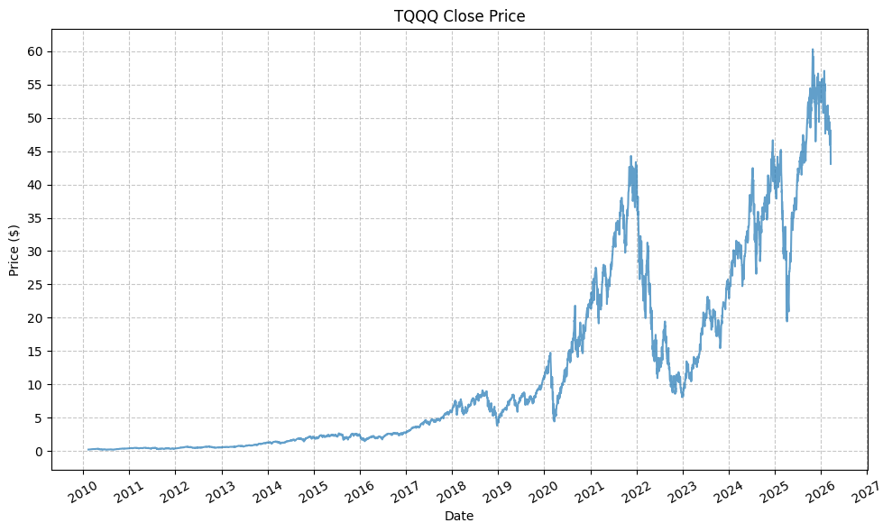
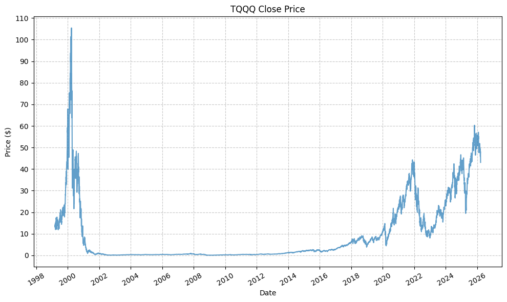
And the plot of the time series of partially adjusted close prices:
plot_time_series(
    df=tqqq,
    plot_start_date=None,
    plot_end_date=None,
    plot_columns=["TQQQ_Close"],
    title="TQQQ Close Price",
    x_label="Date",
    x_format="Year",
    x_tick_spacing=1,
    x_tick_rotation=30,
    y_label="Price ($)",
    y_format="Decimal",
    y_format_decimal_places=0,
    y_tick_spacing="Auto",
    y_tick_rotation=0,
    grid=True,
    legend=False,
    export_plot=False,
    plot_file_name=None,
)
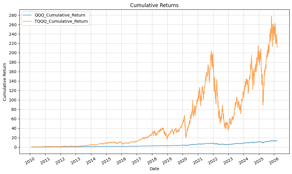
Looking at the close prices doesn’t give us a true picture of the magnitude of the difference in returns due to the leverage. In order to see that, we need to look at the cumulative returns and the drawdowns.
Calculate & Plot Cumulative Returns, Rolling Returns, and Drawdowns (QQQ & TQQQ) #
Next, we will calculate the cumulative returns, rolling returns, and drawdowns. This involves aligning the data to start with the inception of TQQQ. For this excercise, we will not extrapolate the data for QQQ back to 1999, but rather just align the data from the inception of TQQQ in 2010.
etfs = ["QQQ", "TQQQ"]

# Merge dataframes and drop rows with missing values
qqq_tqqq_aligned = tqqq.merge(qqq, left_index=True, right_index=True, how='left')
qqq_tqqq_aligned = qqq_tqqq_aligned.dropna()

# Calculate cumulative returns
for etf in etfs:
    qqq_tqqq_aligned[f"{etf}_Return"] = qqq_tqqq_aligned[f"{etf}_Close"].pct_change()
    qqq_tqqq_aligned[f"{etf}_Cumulative_Return"] = (1 + qqq_tqqq_aligned[f"{etf}_Return"]).cumprod() - 1
    qqq_tqqq_aligned[f"{etf}_Cumulative_Return_Plus_One"] = 1 + qqq_tqqq_aligned[f"{etf}_Cumulative_Return"]
    qqq_tqqq_aligned[f"{etf}_Rolling_Max"] = qqq_tqqq_aligned[f"{etf}_Cumulative_Return_Plus_One"].cummax()
    qqq_tqqq_aligned[f"{etf}_Drawdown"] = qqq_tqqq_aligned[f"{etf}_Cumulative_Return_Plus_One"] / qqq_tqqq_aligned[f"{etf}_Rolling_Max"] - 1
    qqq_tqqq_aligned.drop(columns=[f"{etf}_Cumulative_Return_Plus_One", f"{etf}_Rolling_Max"], inplace=True)

# Define rolling windows in trading days
rolling_windows = {
    '1d': 1,      # 1 day
    '1w': 5,      # 1 week (5 trading days)
    '1m': 21,     # 1 month (~21 trading days)
    '3m': 63,     # 3 months (~63 trading days)
    '6m': 126,    # 6 months (~126 trading days)
    '1y': 252,    # 1 year (~252 trading days)
    '2y': 504,    # 2 years (~504 trading days)
    '3y': 756,    # 3 years (~756 trading days)
    '4y': 1008,   # 4 years (~1008 trading days)
    '5y': 1260,   # 5 years (~1260 trading days)
}

# Calculate rolling returns for each ETF and each window
for etf in etfs:
    for period_name, window in rolling_windows.items():
        qqq_tqqq_aligned[f"{etf}_Rolling_Return_{period_name}"] = (
            qqq_tqqq_aligned[f"{etf}_Close"].pct_change(periods=window)
        )

display(qqq_tqqq_aligned)
| TQQQ_Adj_Close | TQQQ_Close | TQQQ_High | TQQQ_Low | TQQQ_Open | TQQQ_Volume | QQQ_Adj_Close | QQQ_Close | QQQ_High | QQQ_Low | ... | TQQQ_Rolling_Return_1d | TQQQ_Rolling_Return_1w | TQQQ_Rolling_Return_1m | TQQQ_Rolling_Return_3m | TQQQ_Rolling_Return_6m | TQQQ_Rolling_Return_1y | TQQQ_Rolling_Return_2y | TQQQ_Rolling_Return_3y | TQQQ_Rolling_Return_4y | TQQQ_Rolling_Return_5y | |
|---|---|---|---|---|---|---|---|---|---|---|---|---|---|---|---|---|---|---|---|---|---|
| Date | |||||||||||||||||||||
| 2010-02-11 | 0.21 | 0.22 | 0.22 | 0.20 | 0.20 | 6912000 | 37.95 | 43.67 | 43.79 | 42.76 | ... | NaN | NaN | NaN | NaN | NaN | NaN | NaN | NaN | NaN | NaN |
| 2010-02-12 | 0.21 | 0.22 | 0.22 | 0.21 | 0.21 | 17203200 | 38.03 | 43.76 | 43.88 | 43.16 | ... | 0.00 | NaN | NaN | NaN | NaN | NaN | NaN | NaN | NaN | NaN |
| 2010-02-16 | 0.22 | 0.23 | 0.23 | 0.22 | 0.22 | 19238400 | 38.52 | 44.32 | 44.35 | 43.85 | ... | 0.04 | NaN | NaN | NaN | NaN | NaN | NaN | NaN | NaN | NaN |
| 2010-02-17 | 0.22 | 0.23 | 0.23 | 0.23 | 0.23 | 38361600 | 38.73 | 44.57 | 44.57 | 44.26 | ... | 0.02 | NaN | NaN | NaN | NaN | NaN | NaN | NaN | NaN | NaN |
| 2010-02-18 | 0.22 | 0.23 | 0.24 | 0.23 | 0.23 | 77721600 | 38.98 | 44.85 | 44.93 | 44.45 | ... | 0.02 | NaN | NaN | NaN | NaN | NaN | NaN | NaN | NaN | NaN |
| ... | ... | ... | ... | ... | ... | ... | ... | ... | ... | ... | ... | ... | ... | ... | ... | ... | ... | ... | ... | ... | ... |
| 2026-03-16 | 47.46 | 47.46 | 48.27 | 47.18 | 47.37 | 81421500 | 600.38 | 600.38 | 603.86 | 599.11 | ... | 0.03 | -0.04 | -0.02 | -0.15 | -0.02 | 0.64 | 0.60 | 3.36 | 1.25 | 1.22 |
| 2026-03-17 | 48.16 | 48.16 | 48.76 | 47.81 | 48.12 | 74570100 | 603.31 | 603.31 | 605.90 | 601.87 | ... | 0.01 | -0.03 | -0.01 | -0.09 | -0.03 | 0.56 | 0.56 | 3.61 | 1.07 | 1.27 |
| 2026-03-18 | 46.10 | 46.10 | 48.11 | 46.05 | 47.72 | 105059300 | 594.90 | 594.90 | 603.16 | 594.56 | ... | -0.04 | -0.07 | -0.05 | -0.11 | -0.07 | 0.46 | 0.53 | 3.32 | 1.04 | 1.03 |
| 2026-03-19 | 45.69 | 45.69 | 46.32 | 44.30 | 44.87 | 138384900 | 593.02 | 593.02 | 595.80 | 587.08 | ... | -0.01 | -0.02 | -0.07 | -0.13 | -0.07 | 0.53 | 0.52 | 3.01 | 1.16 | 1.06 |
| 2026-03-20 | 43.08 | 43.08 | 45.21 | 42.30 | 45.18 | 137952500 | 582.06 | 582.06 | 591.17 | 578.54 | ... | -0.06 | -0.06 | -0.12 | -0.13 | -0.15 | 0.38 | 0.49 | 2.73 | 1.16 | 0.89 |
4051 rows × 38 columns
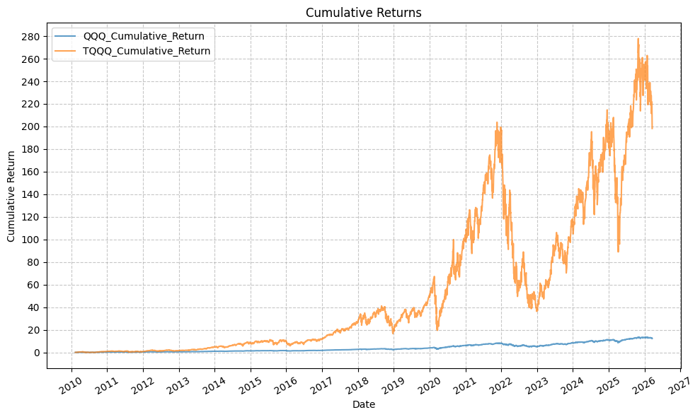
And now the plot for the cumulative returns:
plot_time_series(
    df=qqq_tqqq_aligned,
    plot_start_date=None,
    plot_end_date=None,
    plot_columns=["QQQ_Cumulative_Return", "TQQQ_Cumulative_Return"],
    title="Cumulative Returns",
    x_label="Date",
    x_format="Year",
    x_tick_spacing=1,
    x_tick_rotation=30,
    y_label="Cumulative Return",
    y_format="Decimal",
    y_format_decimal_places=0,
    y_tick_spacing="Auto",
    y_tick_rotation=0,
    grid=True,
    legend=True,
    export_plot=False,
    plot_file_name=None,
)
And the drawdown plot:
plot_time_series(
    df=qqq_tqqq_aligned,
    plot_start_date=None,
    plot_end_date=None,
    plot_columns=["QQQ_Drawdown", "TQQQ_Drawdown"],
    title="Drawdowns",
    x_label="Date",
    x_format="Year",
    x_tick_spacing=1,
    x_tick_rotation=30,
    y_label="Drawdown",
    y_format="Percentage",
    y_format_decimal_places=0,
    y_tick_spacing="Auto",
    y_tick_rotation=0,
    grid=True,
    legend=True,
    export_plot=False,
    plot_file_name=None,
)
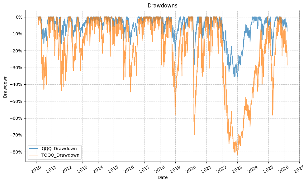
Here is where we truly see the volatility of TQQQ relative to QQQ. In the past 5 years, TQQQ has had drawdowns of 50%, 60%, 70%, and 80%. While it has recovered to make new highs (with the exception of the current ~25% drawdown as of mid-March 2026), very few investors can endure those drawdowns and continue to hold their position. At the same time, we can see from the plot that a ~35% drawdown in QQQ equated to a ~80% drawdown in TQQQ, which is not in fact, 3x. So this tells us (which we already knew) that there is dispersion in the long-term returns relative to the short-term returns between the non-leveraged QQQ and 3x leveraged TQQQ. This idea is well documented in the financial literature as “volatility decay” or “volatility drag”. But, and this is the question we are trying to answer, how significant is this effect over various time horizons?
Summary Statistics (QQQ & TQQQ) #
Looking at the summary statistics further confirms our intuitions about the volatility and drawdowns.
qqq_sum_stats = summary_stats(
    fund_list=["QQQ"],
    df=qqq_tqqq_aligned[["QQQ_Return"]],
    period="Daily",
    use_calendar_days=False,
    excel_export=False,
    pickle_export=False,
    output_confirmation=False,
)

tqqq_sum_stats = summary_stats(
    fund_list=["TQQQ"],
    df=qqq_tqqq_aligned[["TQQQ_Return"]],
    period="Daily",
    use_calendar_days=False,
    excel_export=False,
    pickle_export=False,
    output_confirmation=False,
)

sum_stats = pd.concat([qqq_sum_stats, tqqq_sum_stats])

display(sum_stats)
| Annual Mean Return (Arithmetic) | Annualized Volatility | Annualized Sharpe Ratio | CAGR (Geometric) | Daily Max Return | Daily Max Return (Date) | Daily Min Return | Daily Min Return (Date) | Max Drawdown | Peak | Trough | Recovery Date | Calendar Days to Recovery | MAR Ratio | |
|---|---|---|---|---|---|---|---|---|---|---|---|---|---|---|
| QQQ_Return | 0.18 | 0.21 | 0.89 | 0.17 | 0.12 | 2025-04-09 | -0.12 | 2020-03-16 | -0.36 | 2021-11-19 | 2022-12-28 | 2023-12-15 | 352 | 0.49 |
| TQQQ_Return | 0.52 | 0.61 | 0.85 | 0.39 | 0.35 | 2025-04-09 | -0.34 | 2020-03-16 | -0.82 | 2021-11-19 | 2022-12-28 | 2024-12-11 | 714 | 0.48 |
Note that these statistics are being run on the partially-adjusted close prices, which are not the true returns (due to not accounting for dividends), but they do give us a picture of the relative volatility and drawdowns of the two ETFs. The mean return for TQQQ is much higher than that of QQQ, but the volatility is also much higher, which is consistent with the idea of leverage amplifying both the up-side and down-side. The maximum drawdown for TQQQ is also much higher than that of QQQ, which again confirms our observations from the drawdown plot.
Also note that the daily maximum return for both funds occured during “Liberation Day” and the daily minimum return for both funds occured early on during the COVID-19 pandemic.
Plot Returns & Verify Beta (QQQ & TQQQ) #
Before we look at the rolling returns, let us first verify that the daily returns for TQQQ are in fact ~3x those of QQQ. We can do that by plotting the daily returns for both funds against each other and running a linear regression to see if the beta is indeed ~3.
plot_scatter(
    df=qqq_tqqq_aligned,
    x_plot_column="QQQ_Return",
    y_plot_columns=["TQQQ_Return"],
    title="QQQ & TQQQ Returns",
    x_label="QQQ Return",
    x_format="Decimal",
    x_format_decimal_places=2,
    x_tick_spacing="Auto",
    x_tick_rotation=30,
    y_label="TQQQ Return",
    y_format="Decimal",
    y_format_decimal_places=2,
    y_tick_spacing="Auto",
    y_tick_rotation=0,
    plot_OLS_regression_line=True,
    OLS_column="TQQQ_Return",
    plot_Ridge_regression_line=False,
    Ridge_column=None,
    plot_RidgeCV_regression_line=True,
    RidgeCV_column="TQQQ_Return",
    regression_constant=True,
    grid=True,
    legend=True,
    export_plot=False,
    plot_file_name=None,
)
model = run_linear_regression(
    df=qqq_tqqq_aligned,
    x_plot_column="QQQ_Return",
    y_plot_column="TQQQ_Return",
    regression_model="OLS-statsmodels",
    regression_constant=True,
)

print(model.summary())
                            OLS Regression Results
==============================================================================
Dep. Variable:            TQQQ_Return   R-squared:                       0.997
Model:                            OLS   Adj. R-squared:                  0.997
Method:                 Least Squares   F-statistic:                 1.494e+06
Date:                Mon, 23 Mar 2026   Prob (F-statistic):               0.00
Time:                        21:59:08   Log-Likelihood:                 19431.
No. Observations:                4050   AIC:                        -3.886e+04
Df Residuals:                    4048   BIC:                        -3.884e+04
Df Model:                           1
Covariance Type:            nonrobust
==============================================================================
                 coef    std err          t      P>|t|      [0.025      0.975]
------------------------------------------------------------------------------
const      -8.629e-05   3.14e-05     -2.746      0.006      -0.000   -2.47e-05
QQQ_Return     2.9553      0.002   1222.452      0.000       2.951       2.960
==============================================================================
Omnibus:                     5279.605   Durbin-Watson:                   2.567
Prob(Omnibus):                  0.000   Jarque-Bera (JB):          9197656.554
Skew:                          -6.346   Prob(JB):                         0.00
Kurtosis:                     236.117   Cond. No.                         77.1
==============================================================================

Notes:
[1] Standard Errors assume that the covariance matrix of the errors is correctly specified.
Visually, this plot makes sense and we can see that there is a strong clustering of points, but we double check with the regression, regressing the TQQQ daily return (y) on the QQQ daily return (X).
Given the above result, with a coefficient of 2.96 and an R^2 of 0.997 (based on the statsmodels OLS regression), we can say that TQQQ does in fact return ~3x QQQ. We would also intuitively expect the coefficient to be 0, and it is nearly 0.
Interestingly, the coefficient varies between OLS and Ridge cross-validation, and both are less than 3.
Extrapolate Data (QQQ & TQQQ) #
With the above coefficient, we will now extrapolate the returns of QQQ to backfill the data from the inception of QQQ in 1999 to the inception of TQQQ in 2010 to expand our dataset of returns. For this, we’ll use the coefficient of 2.96 that we found in the regression results above.
# Set leverage multiplier based on regression coefficient
LEVERAGE_MULTIPLIER = model.params[1]

# Merge dataframes and extrapolate return values for QQQ back to 1999 using the leverage multiplier
qqq_tqqq_extrap = qqq[["QQQ_Close"]].merge(tqqq[["TQQQ_Close"]], left_index=True, right_index=True, how='left')

etfs = ["QQQ", "TQQQ"]

# Calculate cumulative returns
for etf in etfs:
    qqq_tqqq_extrap[f"{etf}_Return"] = qqq_tqqq_extrap[f"{etf}_Close"].pct_change()

# Extrapolate TQQQ returns for missing values
qqq_tqqq_extrap["TQQQ_Return"] = qqq_tqqq_extrap["TQQQ_Return"].fillna(LEVERAGE_MULTIPLIER * qqq_tqqq_extrap["QQQ_Return"])

# Find the first valid TQQQ_Close index and value
first_valid_idx = qqq_tqqq_extrap['TQQQ_Close'].first_valid_index()
print(first_valid_idx)
first_valid_price = qqq_tqqq_extrap.loc[first_valid_idx, 'TQQQ_Close']
print(first_valid_price)
2010-02-11 00:00:00
0.21627600491046906
Before we extrapolate, let’s first look at the data we have for QQQ and TQQQ around the inception of TQQQ in 2010:
# Check values around the first valid index
pandas_set_decimal_places(4)
display(qqq_tqqq_extrap.loc["2010-02-08":"2010-02-13"])
| QQQ_Close | TQQQ_Close | QQQ_Return | TQQQ_Return | |
|---|---|---|---|---|
| Date | ||||
| 2010-02-08 | 42.6700 | NaN | -0.0072 | -0.0213 |
| 2010-02-09 | 43.1100 | NaN | 0.0103 | 0.0305 |
| 2010-02-10 | 43.0200 | NaN | -0.0021 | -0.0062 |
| 2010-02-11 | 43.6700 | 0.2163 | 0.0151 | 0.0447 |
| 2010-02-12 | 43.7600 | 0.2172 | 0.0021 | 0.0041 |
Now, backfill the data for the TQQQ close price:
# Iterate through the dataframe backwards
for i in range(qqq_tqqq_extrap.index.get_loc(first_valid_idx) - 1, -1, -1):

    # The return that led to the price the next day
    current_return = qqq_tqqq_extrap.iloc[i + 1]['TQQQ_Return']

    # Get the next day's price
    next_price = qqq_tqqq_extrap.iloc[i + 1]['TQQQ_Close']

    # Price_{t} = Price_{t+1} / (1 + Return_{t})
    qqq_tqqq_extrap.loc[qqq_tqqq_extrap.index[i], 'TQQQ_Close'] = next_price / (1 + current_return)
Finally, confirm the values are correct:
# Confirm values around the first valid index after extrapolation
display(qqq_tqqq_extrap.loc["2010-02-08":"2010-02-13"])
| QQQ_Close | TQQQ_Close | QQQ_Return | TQQQ_Return | |
|---|---|---|---|---|
| Date | ||||
| 2010-02-08 | 42.6700 | 0.2022 | -0.0072 | -0.0213 |
| 2010-02-09 | 43.1100 | 0.2083 | 0.0103 | 0.0305 |
| 2010-02-10 | 43.0200 | 0.2070 | -0.0021 | -0.0062 |
| 2010-02-11 | 43.6700 | 0.2163 | 0.0151 | 0.0447 |
| 2010-02-12 | 43.7600 | 0.2172 | 0.0021 | 0.0041 |
And the complete DataFrame with the extrapolated values:
pandas_set_decimal_places(2)
display(qqq_tqqq_extrap)
| QQQ_Close | TQQQ_Close | QQQ_Return | TQQQ_Return | |
|---|---|---|---|---|
| Date | ||||
| 1999-03-10 | 51.06 | 13.82 | NaN | NaN |
| 1999-03-11 | 51.31 | 14.02 | 0.00 | 0.01 |
| 1999-03-12 | 50.06 | 13.01 | -0.02 | -0.07 |
| 1999-03-15 | 51.50 | 14.11 | 0.03 | 0.08 |
| 1999-03-16 | 51.94 | 14.47 | 0.01 | 0.03 |
| ... | ... | ... | ... | ... |
| 2026-03-16 | 600.38 | 47.46 | 0.01 | 0.03 |
| 2026-03-17 | 603.31 | 48.16 | 0.00 | 0.01 |
| 2026-03-18 | 594.90 | 46.10 | -0.01 | -0.04 |
| 2026-03-19 | 593.02 | 45.69 | -0.00 | -0.01 |
| 2026-03-20 | 582.06 | 43.08 | -0.02 | -0.06 |
6800 rows × 4 columns
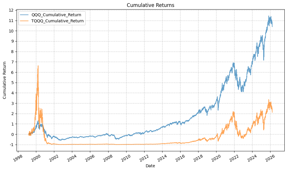
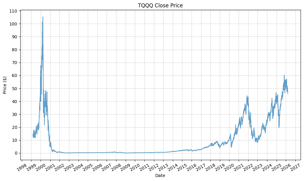
After the extrapolation, we now have the following plots for the prices, cumulative returns, and drawdowns:
etfs = ["QQQ", "TQQQ"]

# Calculate cumulative returns
for etf in etfs:
    qqq_tqqq_extrap[f"{etf}_Return"] = qqq_tqqq_extrap[f"{etf}_Close"].pct_change()
    qqq_tqqq_extrap[f"{etf}_Cumulative_Return"] = (1 + qqq_tqqq_extrap[f"{etf}_Return"]).cumprod() - 1
    qqq_tqqq_extrap[f"{etf}_Cumulative_Return_Plus_One"] = 1 + qqq_tqqq_extrap[f"{etf}_Cumulative_Return"]
    qqq_tqqq_extrap[f"{etf}_Rolling_Max"] = qqq_tqqq_extrap[f"{etf}_Cumulative_Return_Plus_One"].cummax()
    qqq_tqqq_extrap[f"{etf}_Drawdown"] = qqq_tqqq_extrap[f"{etf}_Cumulative_Return_Plus_One"] / qqq_tqqq_extrap[f"{etf}_Rolling_Max"] - 1
    qqq_tqqq_extrap.drop(columns=[f"{etf}_Cumulative_Return_Plus_One", f"{etf}_Rolling_Max"], inplace=True)
plot_time_series(
    df=qqq_tqqq_extrap,
    plot_start_date=None,
    plot_end_date=None,
    plot_columns=["QQQ_Close"],
    title="QQQ Close Price",
    x_label="Date",
    x_format="Year",
    x_tick_spacing=2,
    x_tick_rotation=30,
    y_label="Price ($)",
    y_format="Decimal",
    y_format_decimal_places=0,
    y_tick_spacing="Auto",
    y_tick_rotation=0,
    grid=True,
    legend=False,
    export_plot=False,
    plot_file_name=None,
)

plot_time_series(
    df=qqq_tqqq_extrap,
    plot_start_date=None,
    plot_end_date=None,
    plot_columns=["TQQQ_Close"],
    title="TQQQ Close Price",
    x_label="Date",
    x_format="Year",
    x_tick_spacing=2,
    x_tick_rotation=30,
    y_label="Price ($)",
    y_format="Decimal",
    y_format_decimal_places=0,
    y_tick_spacing="Auto",
    y_tick_rotation=0,
    grid=True,
    legend=False,
    export_plot=False,
    plot_file_name=None,
)
plot_time_series(
    df=qqq_tqqq_extrap,
    plot_start_date=None,
    plot_end_date=None,
    plot_columns=["QQQ_Cumulative_Return", "TQQQ_Cumulative_Return"],
    title="Cumulative Returns",
    x_label="Date",
    x_format="Year",
    x_tick_spacing=2,
    x_tick_rotation=30,
    y_label="Cumulative Return",
    y_format="Decimal",
    y_format_decimal_places=0,
    y_tick_spacing="Auto",
    y_tick_rotation=0,
    grid=True,
    legend=True,
    export_plot=False,
    plot_file_name=None,
)
plot_time_series(
    df=qqq_tqqq_extrap,
    plot_start_date=None,
    plot_end_date=None,
    plot_columns=["QQQ_Drawdown", "TQQQ_Drawdown"],
    title="Drawdowns",
    x_label="Date",
    x_format="Year",
    x_tick_spacing=2,
    x_tick_rotation=30,
    y_label="Drawdown",
    y_format="Percentage",
    y_format_decimal_places=0,
    y_tick_spacing="Auto",
    y_tick_rotation=0,
    grid=True,
    legend=True,
    export_plot=False,
    plot_file_name=None,
)

qqq_extrap_sum_stats = summary_stats(
    fund_list=["QQQ"],
    df=qqq_tqqq_extrap[["QQQ_Return"]],
    period="Daily",
    use_calendar_days=False,
    excel_export=False,
    pickle_export=False,
    output_confirmation=False,
)

tqqq_extrap_sum_stats = summary_stats(
    fund_list=["TQQQ"],
    df=qqq_tqqq_extrap[["TQQQ_Return"]],
    period="Daily",
    use_calendar_days=False,
    excel_export=False,
    pickle_export=False,
    output_confirmation=False,
)

sum_stats = pd.concat([qqq_sum_stats, tqqq_sum_stats, qqq_extrap_sum_stats, tqqq_extrap_sum_stats])
sum_stats.index = ["QQQ (2010 - Present)", "TQQQ (2010 - Present)", "QQQ (1999 - Present)", "TQQQ Extrapolated (1999 - Present)"]

display(sum_stats)
| Annual Mean Return (Arithmetic) | Annualized Volatility | Annualized Sharpe Ratio | CAGR (Geometric) | Daily Max Return | Daily Max Return (Date) | Daily Min Return | Daily Min Return (Date) | Max Drawdown | Peak | Trough | Recovery Date | Calendar Days to Recovery | MAR Ratio | |
|---|---|---|---|---|---|---|---|---|---|---|---|---|---|---|
| QQQ (2010 - Present) | 0.18 | 0.21 | 0.89 | 0.17 | 0.12 | 2025-04-09 | -0.12 | 2020-03-16 | -0.36 | 2021-11-19 | 2022-12-28 | 2023-12-15 | 352.00 | 0.49 |
| TQQQ (2010 - Present) | 0.52 | 0.61 | 0.85 | 0.39 | 0.35 | 2025-04-09 | -0.34 | 2020-03-16 | -0.82 | 2021-11-19 | 2022-12-28 | 2024-12-11 | 714.00 | 0.48 |
| QQQ (1999 - Present) | 0.13 | 0.27 | 0.47 | 0.09 | 0.17 | 2001-01-03 | -0.12 | 2020-03-16 | -0.83 | 2000-03-27 | 2002-10-09 | 2016-09-06 | 5081.00 | 0.11 |
| TQQQ Extrapolated (1999 - Present) | 0.36 | 0.80 | 0.45 | 0.04 | 0.50 | 2001-01-03 | -0.34 | 2020-03-16 | -1.00 | 2000-03-27 | 2009-03-09 | NaT | NaN | 0.04 |
A few quick comments before we look at rolling returns:
- The cumulative return for TQQQ is less than that of QQQ - which is starkly different from the plot beginning in 2010 at the inception of TQQQ. So the return path really matters here.
- The drawdown for TQQQ is nearly 100%… which also represents nearly a total loss of capital for any allocation to the extrap-TQQQ. Furthermore, as we walk forward through time (2002, 2003, … etc.), there is really no reason to believe that the returns would ever recover (even partially). So while we can look at the rolling returns and see how they compare to the 3x return of QQQ, we should keep in mind that the drawdown post-1999 is so severe that it would be very difficult for any investor to hold through it.
- The recovery time for QQQ was more than 5,000 days, or ~14 years. Note that this is calendar days, not trading days. While returns have been great for QQQ since 2016, the 14 year dry spell is a reminder of just how large the tech bubble was.
- The extrapolated TQQQ data remains in a drawdown and has never recovered to make new highs (as of March 2026).
Plot Rolling Returns (QQQ & TQQQ) #
Next, we will consider the following:
- Histogram and scatter plots of the rolling returns of QQQ and TQQQ
- Regressions to establish a “leverage factor” for the rolling returns
- The deviation from a 3x return for each time period
For this set of regressions, we will also allow the constant. First, we need the rolling returns for various time periods:
# Define rolling windows in trading days
rolling_windows = {
    '1d': 1,      # 1 day
    '1w': 5,      # 1 week (5 trading days)
    '1m': 21,     # 1 month (~21 trading days)
    '3m': 63,     # 3 months (~63 trading days)
    '6m': 126,    # 6 months (~126 trading days)
    '1y': 252,    # 1 year (~252 trading days)
    '2y': 504,    # 2 years (~504 trading days)
    '3y': 756,    # 3 years (~756 trading days)
    '4y': 1008,   # 4 years (~1008 trading days)
    '5y': 1260,   # 5 years (~1260 trading days)
}

# Calculate rolling returns for each ETF and each window
for etf in etfs:
    for period_name, window in rolling_windows.items():
        qqq_tqqq_extrap[f"{etf}_Rolling_Return_{period_name}"] = (
            qqq_tqqq_extrap[f"{etf}_Close"].pct_change(periods=window)
        )
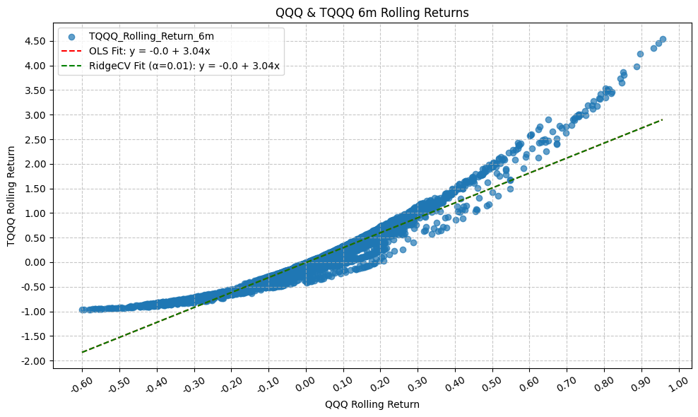
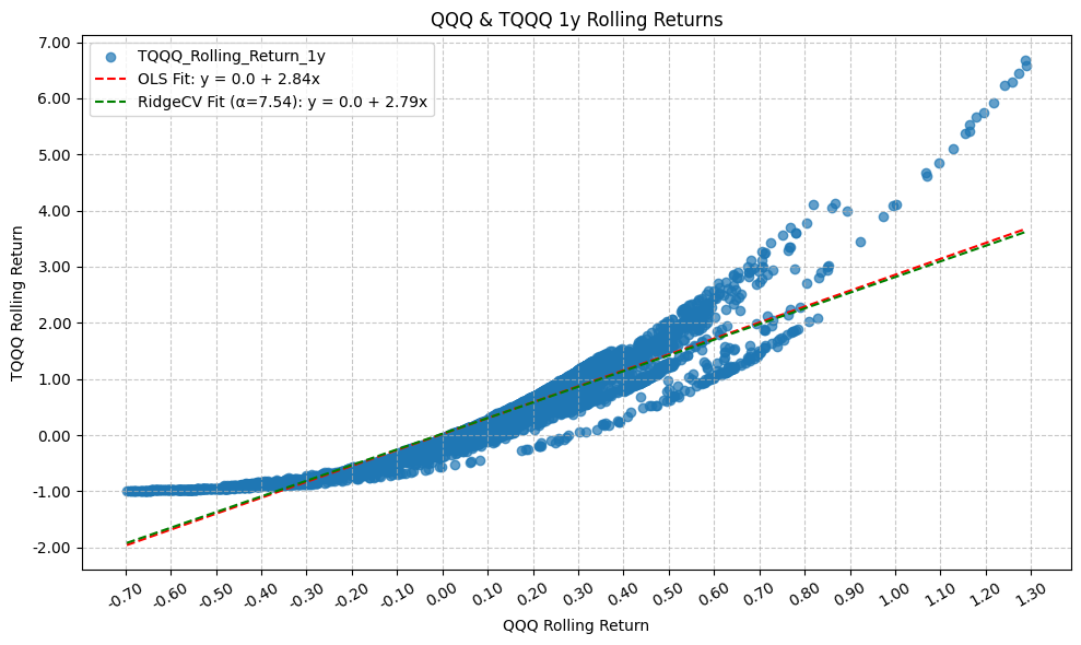
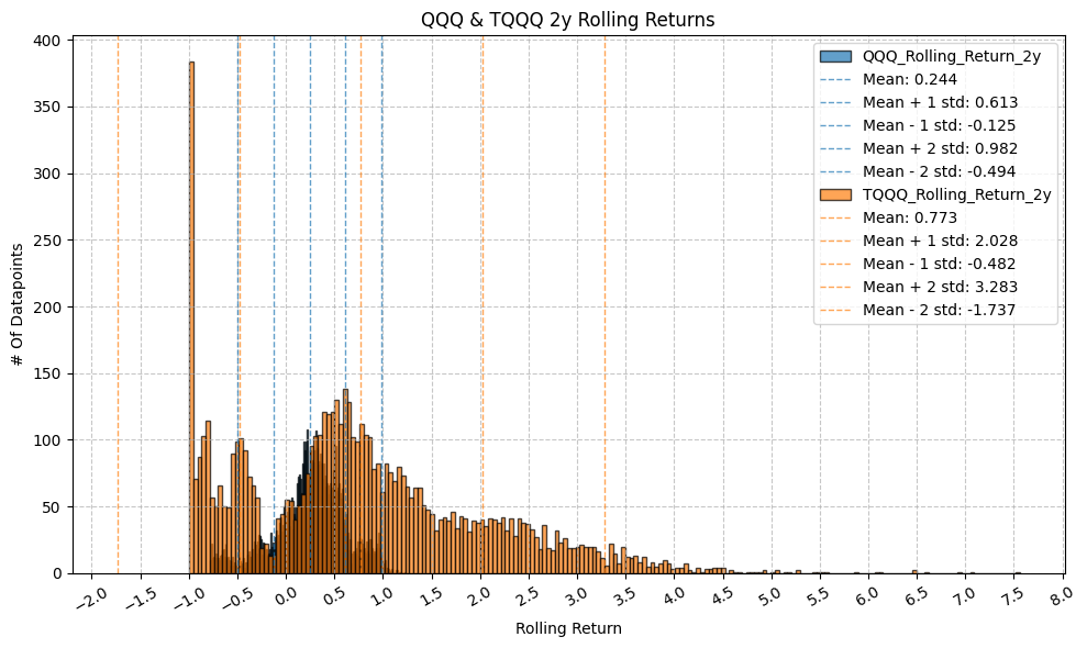
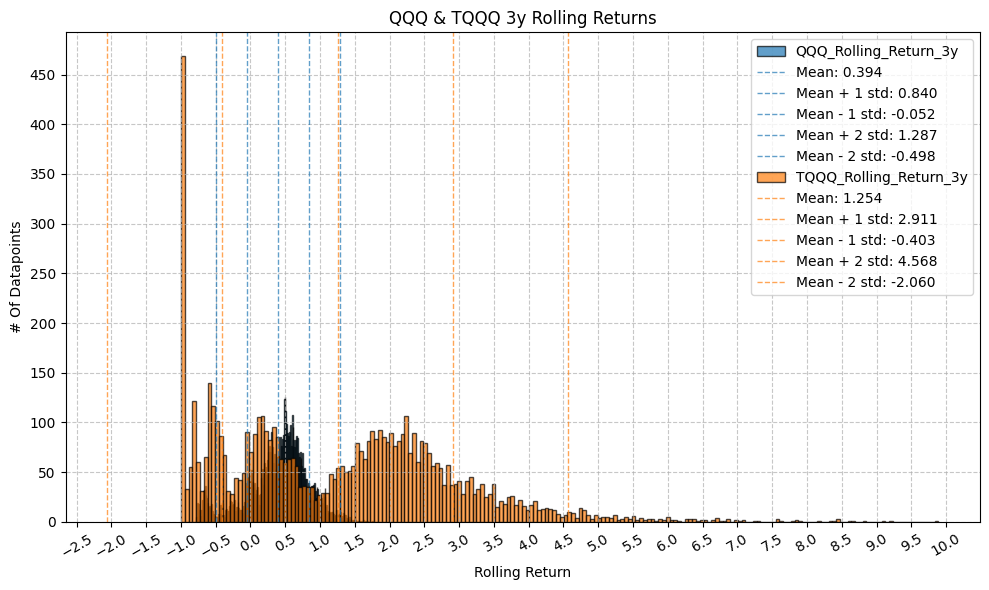
This gives us the following series of histograms, scatter plots, and regression model results:
# Create a dataframe to hold rolling returns stats
rolling_returns_stats = pd.DataFrame()
for period_name, window in rolling_windows.items():
plot_histogram(
df=qqq_tqqq_extrap,
plot_columns=[f"QQQ_Rolling_Return_{period_name}", f"TQQQ_Rolling_Return_{period_name}"],
title=f"QQQ & TQQQ {period_name} Rolling Returns",
x_label="Rolling Return",
x_tick_spacing="Auto",
x_tick_rotation=30,
y_label="# Of Datapoints",
y_tick_spacing="Auto",
y_tick_rotation=0,
grid=True,
legend=True,
export_plot=False,
plot_file_name=None,
)
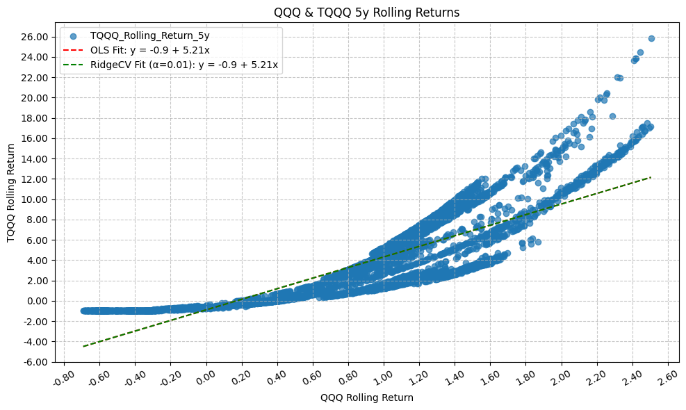
plot_scatter(
df=qqq_tqqq_extrap,
x_plot_column=f"QQQ_Rolling_Return_{period_name}",
y_plot_columns=[f"TQQQ_Rolling_Return_{period_name}"],
title=f"QQQ & TQQQ {period_name} Rolling Returns",
x_label="QQQ Rolling Return",
x_format="Decimal",
x_format_decimal_places=2,
x_tick_spacing="Auto",
x_tick_rotation=30,
y_label="TQQQ Rolling Return",
y_format="Decimal",
y_format_decimal_places=2,
y_tick_spacing="Auto",
y_tick_rotation=0,
plot_OLS_regression_line=True,
OLS_column=f"TQQQ_Rolling_Return_{period_name}",
plot_Ridge_regression_line=False,
Ridge_column=None,
plot_RidgeCV_regression_line=True,
RidgeCV_column=f"TQQQ_Rolling_Return_{period_name}",
regression_constant=True,
grid=True,
legend=True,
export_plot=False,
plot_file_name=None,
)
# Run OLS regression with statsmodels
model = run_linear_regression(
df=qqq_tqqq_extrap,
x_plot_column=f"QQQ_Rolling_Return_{period_name}",
y_plot_column=f"TQQQ_Rolling_Return_{period_name}",
regression_model="OLS-statsmodels",
regression_constant=True,
)
print(model.summary())
# Add the regression results to the rolling returns stats dataframe
intercept = model.params[0]
intercept_pvalue = model.pvalues[0] # p-value for Intercept
slope = model.params[1]
slope_pvalue = model.pvalues[1] # p-value for QQQ_Return
r_squared = model.rsquared
# Calc skew
return_ratio = qqq_tqqq_extrap[f'TQQQ_Rolling_Return_{period_name}'] / qqq_tqqq_extrap[f'QQQ_Rolling_Return_{period_name}']
skew = return_ratio.skew()
# Calc conditional symmetry
up_markets = qqq_tqqq_extrap[qqq_tqqq_extrap[f'QQQ_Rolling_Return_{period_name}'] > 0]
down_markets = qqq_tqqq_extrap[qqq_tqqq_extrap[f'QQQ_Rolling_Return_{period_name}'] <= 0]
avg_beta_up = (up_markets[f'TQQQ_Rolling_Return_{period_name}'] / up_markets[f'QQQ_Rolling_Return_{period_name}']).mean()
avg_beta_down = (down_markets[f'TQQQ_Rolling_Return_{period_name}'] / down_markets[f'QQQ_Rolling_Return_{period_name}']).mean()
asymmetry = avg_beta_up - avg_beta_down
rolling_returns_slope_int = pd.DataFrame({
"Period": period_name,
"Intercept": [intercept],
# "Intercept_PValue": [intercept_pvalue],
"Slope": [slope],
# "Slope_PValue": [slope_pvalue],
"R_Squared": [r_squared],
"Return Skew": [skew],
"Average Upside Beta": [avg_beta_up],
"Average Downside Beta": [avg_beta_down],
"Asymmetry": [asymmetry]
})
rolling_returns_stats = pd.concat([rolling_returns_stats, rolling_returns_slope_int])
                              OLS Regression Results
==================================================================================
Dep. Variable:     TQQQ_Rolling_Return_1d   R-squared:                       0.999
Model:                                OLS   Adj. R-squared:                  0.999
Method:                     Least Squares   F-statistic:                 7.219e+06
Date:                    Mon, 23 Mar 2026   Prob (F-statistic):               0.00
Time:                            21:59:12   Log-Likelihood:                 34378.
No. Observations:                    6799   AIC:                        -6.875e+04
Df Residuals:                        6797   BIC:                        -6.874e+04
Df Model:                               1
Covariance Type:                nonrobust
=========================================================================================
                            coef    std err          t      P>|t|      [0.025      0.975]
-----------------------------------------------------------------------------------------
const                 -5.138e-05   1.87e-05     -2.748      0.006    -8.8e-05   -1.47e-05
QQQ_Rolling_Return_1d     2.9552      0.001   2686.888      0.000       2.953       2.957
==============================================================================
Omnibus:                    10196.347   Durbin-Watson:                   2.565
Prob(Omnibus):                  0.000   Jarque-Bera (JB):         43934832.029
Skew:                          -8.279   Prob(JB):                         0.00
Kurtosis:                     396.463   Cond. No.                         58.8
==============================================================================

Notes:
[1] Standard Errors assume that the covariance matrix of the errors is correctly specified.
                              OLS Regression Results
==================================================================================
Dep. Variable:     TQQQ_Rolling_Return_1w   R-squared:                       0.994
Model:                                OLS   Adj. R-squared:                  0.994
Method:                     Least Squares   F-statistic:                 1.117e+06
Date:                    Mon, 23 Mar 2026   Prob (F-statistic):               0.00
Time:                            21:59:14   Log-Likelihood:                 23171.
No. Observations:                    6795   AIC:                        -4.634e+04
Df Residuals:                        6793   BIC:                        -4.632e+04
Df Model:                               1
Covariance Type:                nonrobust
=========================================================================================
                            coef    std err          t      P>|t|      [0.025      0.975]
-----------------------------------------------------------------------------------------
const                    -0.0008   9.72e-05     -8.359      0.000      -0.001      -0.001
QQQ_Rolling_Return_1w     2.9525      0.003   1056.784      0.000       2.947       2.958
==============================================================================
Omnibus:                     2840.677   Durbin-Watson:                   0.932
Prob(Omnibus):                  0.000   Jarque-Bera (JB):           565062.032
Skew:                          -0.863   Prob(JB):                         0.00
Kurtosis:                      47.641   Cond. No.                         28.8
==============================================================================

Notes:
[1] Standard Errors assume that the covariance matrix of the errors is correctly specified.
                              OLS Regression Results
==================================================================================
Dep. Variable:     TQQQ_Rolling_Return_1m   R-squared:                       0.982
Model:                                OLS   Adj. R-squared:                  0.982
Method:                     Least Squares   F-statistic:                 3.698e+05
Date:                    Mon, 23 Mar 2026   Prob (F-statistic):               0.00
Time:                            21:59:16   Log-Likelihood:                 14865.
No. Observations:                    6779   AIC:                        -2.973e+04
Df Residuals:                        6777   BIC:                        -2.971e+04
Df Model:                               1
Covariance Type:                nonrobust
=========================================================================================
                            coef    std err          t      P>|t|      [0.025      0.975]
-----------------------------------------------------------------------------------------
const                    -0.0037      0.000    -11.098      0.000      -0.004      -0.003
QQQ_Rolling_Return_1m     2.9306      0.005    608.073      0.000       2.921       2.940
==============================================================================
Omnibus:                     1630.144   Durbin-Watson:                   0.296
Prob(Omnibus):                  0.000   Jarque-Bera (JB):            69176.713
Skew:                           0.358   Prob(JB):                         0.00
Kurtosis:                      18.633   Cond. No.                         14.7
==============================================================================

Notes:
[1] Standard Errors assume that the covariance matrix of the errors is correctly specified.
                              OLS Regression Results
==================================================================================
Dep. Variable:     TQQQ_Rolling_Return_3m   R-squared:                       0.958
Model:                                OLS   Adj. R-squared:                  0.958
Method:                     Least Squares   F-statistic:                 1.551e+05
Date:                    Mon, 23 Mar 2026   Prob (F-statistic):               0.00
Time:                            21:59:18   Log-Likelihood:                 7953.7
No. Observations:                    6737   AIC:                        -1.590e+04
Df Residuals:                        6735   BIC:                        -1.589e+04
Df Model:                               1
Covariance Type:                nonrobust
=========================================================================================
                            coef    std err          t      P>|t|      [0.025      0.975]
-----------------------------------------------------------------------------------------
const                    -0.0083      0.001     -8.874      0.000      -0.010      -0.006
QQQ_Rolling_Return_3m     2.9849      0.008    393.789      0.000       2.970       3.000
==============================================================================
Omnibus:                     3466.652   Durbin-Watson:                   0.105
Prob(Omnibus):                  0.000   Jarque-Bera (JB):            79721.487
Skew:                           1.963   Prob(JB):                         0.00
Kurtosis:                      19.389   Cond. No.                         8.38
==============================================================================

Notes:
[1] Standard Errors assume that the covariance matrix of the errors is correctly specified.
                              OLS Regression Results
==================================================================================
Dep. Variable:     TQQQ_Rolling_Return_6m   R-squared:                       0.916
Model:                                OLS   Adj. R-squared:                  0.916
Method:                     Least Squares   F-statistic:                 7.252e+04
Date:                    Mon, 23 Mar 2026   Prob (F-statistic):               0.00
Time:                            21:59:19   Log-Likelihood:                 2613.7
No. Observations:                    6674   AIC:                            -5223.
Df Residuals:                        6672   BIC:                            -5210.
Df Model:                               1
Covariance Type:                nonrobust
=========================================================================================
                            coef    std err          t      P>|t|      [0.025      0.975]
-----------------------------------------------------------------------------------------
const                    -0.0097      0.002     -4.549      0.000      -0.014      -0.005
QQQ_Rolling_Return_6m     3.0397      0.011    269.293      0.000       3.018       3.062
==============================================================================
Omnibus:                     3659.091   Durbin-Watson:                   0.056
Prob(Omnibus):                  0.000   Jarque-Bera (JB):            60225.360
Skew:                           2.263   Prob(JB):                         0.00
Kurtosis:                      17.003   Cond. No.                         5.66
==============================================================================

Notes:
[1] Standard Errors assume that the covariance matrix of the errors is correctly specified.

                              OLS Regression Results
==================================================================================
Dep. Variable:     TQQQ_Rolling_Return_1y   R-squared:                       0.880
Model:                                OLS   Adj. R-squared:                  0.880
Method:                     Least Squares   F-statistic:                 4.786e+04
Date:                    Mon, 23 Mar 2026   Prob (F-statistic):               0.00
Time:                            21:59:21   Log-Likelihood:                -892.41
No. Observations:                    6548   AIC:                             1789.
Df Residuals:                        6546   BIC:                             1802.
Df Model:                               1
Covariance Type:                nonrobust
=========================================================================================
                            coef    std err          t      P>|t|      [0.025      0.975]
-----------------------------------------------------------------------------------------
const                     0.0189      0.004      5.003      0.000       0.012       0.026
QQQ_Rolling_Return_1y     2.8372      0.013    218.775      0.000       2.812       2.863
==============================================================================
Omnibus:                     3497.781   Durbin-Watson:                   0.037
Prob(Omnibus):                  0.000   Jarque-Bera (JB):            68281.594
Skew:                           2.124   Prob(JB):                         0.00
Kurtosis:                      18.239   Cond. No.                         3.85
==============================================================================

Notes:
[1] Standard Errors assume that the covariance matrix of the errors is correctly specified.

                              OLS Regression Results
==================================================================================
Dep. Variable:     TQQQ_Rolling_Return_2y   R-squared:                       0.848
Model:                                OLS   Adj. R-squared:                  0.848
Method:                     Least Squares   F-statistic:                 3.521e+04
Date:                    Mon, 23 Mar 2026   Prob (F-statistic):               0.00
Time:                            21:59:22   Log-Likelihood:                -4425.9
No. Observations:                    6296   AIC:                             8856.
Df Residuals:                        6294   BIC:                             8869.
Df Model:                               1
Covariance Type:                nonrobust
=========================================================================================
                            coef    std err          t      P>|t|      [0.025      0.975]
-----------------------------------------------------------------------------------------
const                     0.0092      0.007      1.243      0.214      -0.005       0.024
QQQ_Rolling_Return_2y     3.1310      0.017    187.631      0.000       3.098       3.164
==============================================================================
Omnibus:                     1596.134   Durbin-Watson:                   0.019
Prob(Omnibus):                  0.000   Jarque-Bera (JB):             4146.775
Skew:                           1.367   Prob(JB):                         0.00
Kurtosis:                       5.886   Cond. No.                         2.89
==============================================================================

Notes:
[1] Standard Errors assume that the covariance matrix of the errors is correctly specified.
                              OLS Regression Results
==================================================================================
Dep. Variable:     TQQQ_Rolling_Return_3y   R-squared:                       0.805
Model:                                OLS   Adj. R-squared:                  0.804
Method:                     Least Squares   F-statistic:                 2.487e+04
Date:                    Mon, 23 Mar 2026   Prob (F-statistic):               0.00
Time:                            21:59:24   Log-Likelihood:                -6694.8
No. Observations:                    6044   AIC:                         1.339e+04
Df Residuals:                        6042   BIC:                         1.341e+04
Df Model:                               1
Covariance Type:                nonrobust
=========================================================================================
                            coef    std err          t      P>|t|      [0.025      0.975]
-----------------------------------------------------------------------------------------
const                    -0.0599      0.013     -4.764      0.000      -0.085      -0.035
QQQ_Rolling_Return_3y     3.3318      0.021    157.695      0.000       3.290       3.373
==============================================================================
Omnibus:                      858.024   Durbin-Watson:                   0.015
Prob(Omnibus):                  0.000   Jarque-Bera (JB):             1472.819
Skew:                           0.940   Prob(JB):                         0.00
Kurtosis:                       4.521   Cond. No.                         2.66
==============================================================================

Notes:
[1] Standard Errors assume that the covariance matrix of the errors is correctly specified.
                              OLS Regression Results
==================================================================================
Dep. Variable:     TQQQ_Rolling_Return_4y   R-squared:                       0.781
Model:                                OLS   Adj. R-squared:                  0.781
Method:                     Least Squares   F-statistic:                 2.064e+04
Date:                    Mon, 23 Mar 2026   Prob (F-statistic):               0.00
Time:                            21:59:26   Log-Likelihood:                -8794.2
No. Observations:                    5792   AIC:                         1.759e+04
Df Residuals:                        5790   BIC:                         1.761e+04
Df Model:                               1
Covariance Type:                nonrobust
=========================================================================================
                            coef    std err          t      P>|t|      [0.025      0.975]
-----------------------------------------------------------------------------------------
const                    -0.2930      0.021    -13.695      0.000      -0.335      -0.251
QQQ_Rolling_Return_4y     3.9329      0.027    143.656      0.000       3.879       3.987
==============================================================================
Omnibus:                      200.096   Durbin-Watson:                   0.010
Prob(Omnibus):                  0.000   Jarque-Bera (JB):              104.261
Skew:                           0.140   Prob(JB):                     2.29e-23
Kurtosis:                       2.405   Cond. No.                         2.66
==============================================================================

Notes:
[1] Standard Errors assume that the covariance matrix of the errors is correctly specified.
                              OLS Regression Results
==================================================================================
Dep. Variable:     TQQQ_Rolling_Return_5y   R-squared:                       0.743
Model:                                OLS   Adj. R-squared:                  0.743
Method:                     Least Squares   F-statistic:                 1.598e+04
Date:                    Mon, 23 Mar 2026   Prob (F-statistic):               0.00
Time:                            21:59:28   Log-Likelihood:                -12084.
No. Observations:                    5540   AIC:                         2.417e+04
Df Residuals:                        5538   BIC:                         2.418e+04
Df Model:                               1
Covariance Type:                nonrobust
=========================================================================================
                            coef    std err          t      P>|t|      [0.025      0.975]
-----------------------------------------------------------------------------------------
const                    -0.8875      0.044    -19.973      0.000      -0.975      -0.800
QQQ_Rolling_Return_5y     5.2051      0.041    126.424      0.000       5.124       5.286
==============================================================================
Omnibus:                      315.142   Durbin-Watson:                   0.009
Prob(Omnibus):                  0.000   Jarque-Bera (JB):              460.565
Skew:                           0.499   Prob(JB):                    9.76e-101
Kurtosis:                       4.000   Cond. No.                         2.73
==============================================================================

Notes:
[1] Standard Errors assume that the covariance matrix of the errors is correctly specified.
You’re welcome to digest each plot, but here’s my observations on the above results:
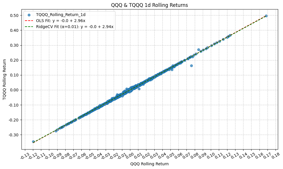
- 1d: TQQQ tracks QQQ as expected (it’s a 3x daily return leveraged ETF after all), with a regression coefficient of 2.96 and an R^2 of 0.997, and we extrapolated half the data with the same coefficient.
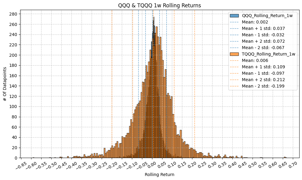
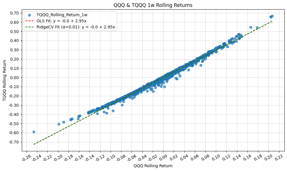
- 1w: Essentially the same as above. A few outliers, but the regression coefficient is still 2.95 with an R^2 of 0.994. We see a slight skew toward the positive in the rolling returns.
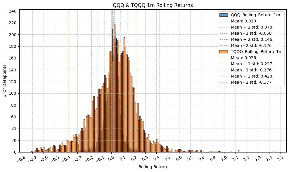
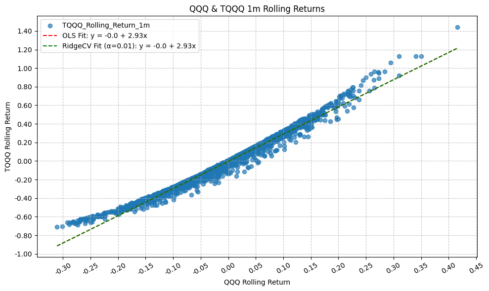
- 1m: The skew toward the positive is more pronounced, and we see more outliers. The regression coefficient has decreased to 2.93 and the R^2 has dropped to 0.98, which is still very high, but we are starting to see some dispersion in the returns.
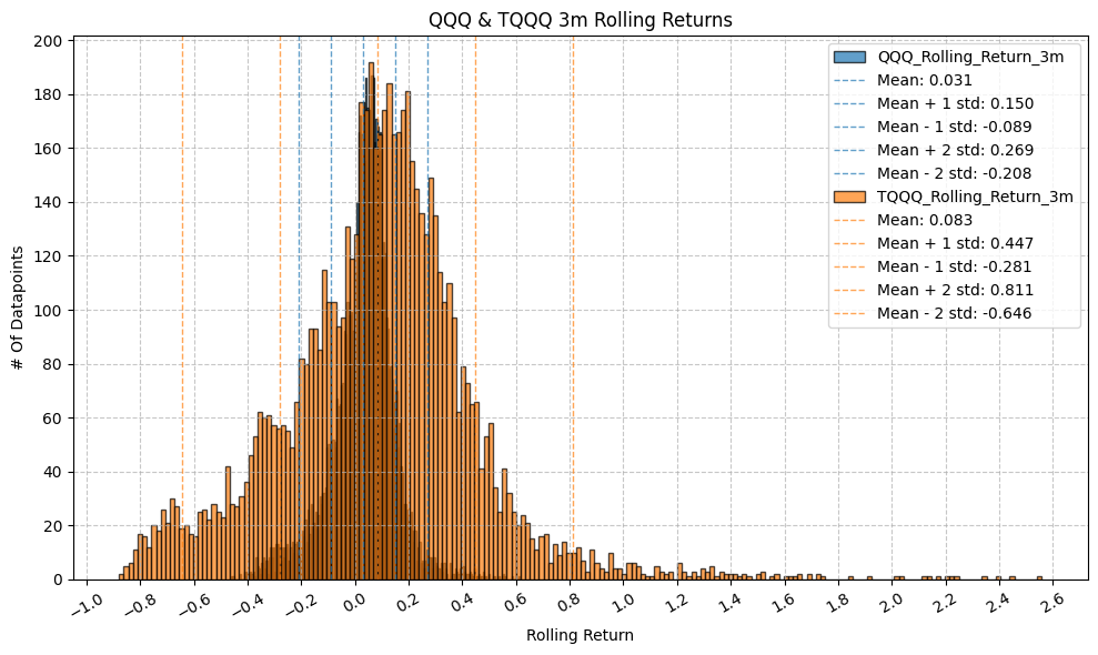
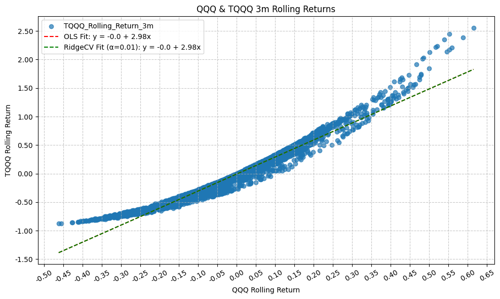
- 3m: The skew toward the positive is even more pronounced, and we see even more outliers. The regression coefficient has increased, to 2.98 and the R^2 has dropped to 0.96.
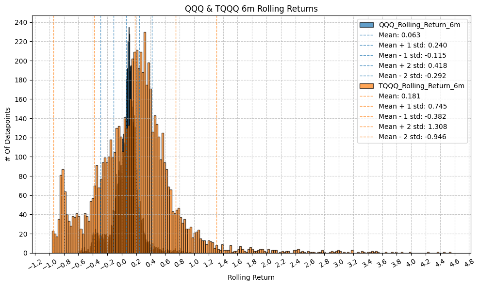
- 6m: The skew toward the positive is very pronounced, and we see a significant number of outliers with pronounced curvanture in the plot. The regression coefficient has increased again, to 3.4 and the R^2 has dropped to 0.92.
- 1y: At this point, based on the plot and the regression results, we can start to see that the returns of TQQQ are no longer tracking 3x the returns of QQQ as closely as they did in the shorter time periods. The regression coefficient has is now 2.84 and the R^2 has dropped to 0.88.
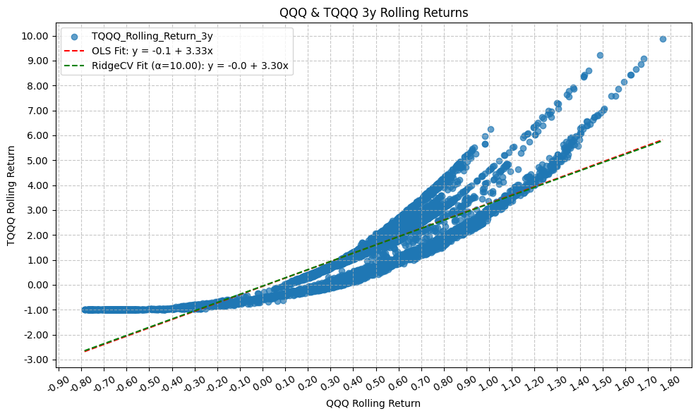
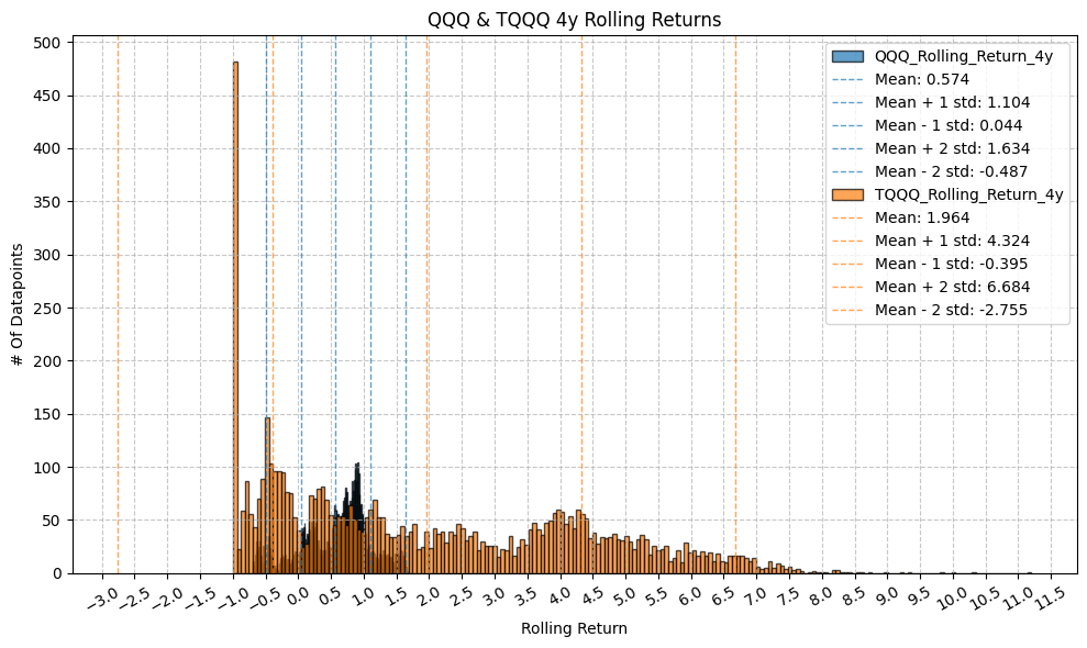
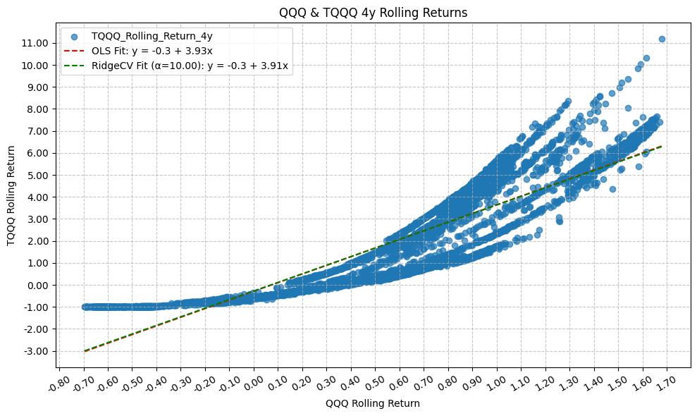
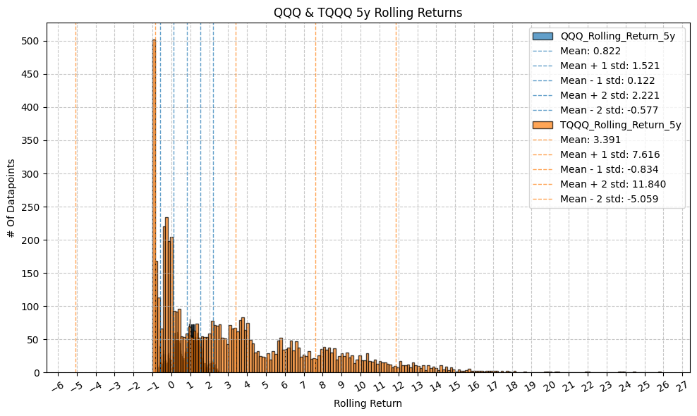
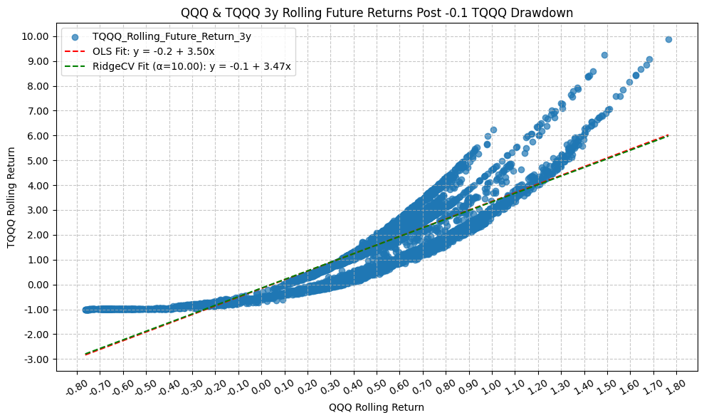
- 4y and 5y: We can see that there are periods where the rolling returns of TQQQ are significantly higher and lower than 3x the returns of QQQ, which is consistent with the idea of volatility decay.
For 4y, based on the regression results, we see that if the rolling return of QQQ was 0, then we would expect a return of -0.30 for TQQQ.
$$ r_{TQQQ} = -0.30 + 3.93 \times r_{QQQ} = -0.30 + 3.93 \times 0 = -0.30 $$
On the other end of the spectrum, if the rolling return of QQQ was 1, then we would expect a return of:
$$ r_{TQQQ} = -0.30 + 3.93 \times r_{QQQ} = -0.30 + 3.93 \times 1 = 3.63 $$
In general, the positive skew of the rolling returns of TQQQ relative to QQQ is related to the general postive return performance of QQQ. With sustained positive returns, the leverage effect of TQQQ will amplify those returns, leading to a positive skew. However, during periods of negative returns for QQQ, the leverage effect will also amplify those losses, leading to a negative skew, and to the limit of a cumulative return of -1, or a 100% loss. The overall skewness of the rolling returns will depend on the balance of these positive and negative periods.
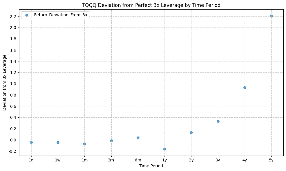
Rolling Returns Deviation (QQQ & TQQQ) #
Next, we will the rolling returns deviation from the expected 3x return for each time period. This will give us a better picture of the volatility decay effect and how it changes over different time horizons.
rolling_returns_stats["Return_Deviation_From_3x"] = rolling_returns_stats["Slope"] - 3.0
pandas_set_decimal_places(3)
display(rolling_returns_stats.set_index("Period"))
| Intercept | Slope | R_Squared | Return Skew | Average Upside Beta | Average Downside Beta | Asymmetry | Return_Deviation_From_3x | |
|---|---|---|---|---|---|---|---|---|
| Period | ||||||||
| 1d | -0.000 | 2.955 | 0.999 | NaN | 2.957 | NaN | NaN | -0.045 |
| 1w | -0.001 | 2.952 | 0.994 | NaN | 2.553 | NaN | NaN | -0.048 |
| 1m | -0.004 | 2.931 | 0.982 | NaN | 2.208 | NaN | NaN | -0.069 |
| 3m | -0.008 | 2.985 | 0.958 | NaN | 1.994 | -inf | inf | -0.015 |
| 6m | -0.010 | 3.040 | 0.916 | -8.728 | 1.478 | 5.417 | -3.939 | 0.040 |
| 1y | 0.019 | 2.837 | 0.880 | NaN | 1.223 | -inf | inf | -0.163 |
| 2y | 0.009 | 3.131 | 0.848 | 36.170 | 1.393 | 12.342 | -10.948 | 0.131 |
| 3y | -0.060 | 3.332 | 0.805 | NaN | -0.088 | -inf | inf | 0.332 |
| 4y | -0.293 | 3.933 | 0.781 | 19.562 | 1.759 | 7.212 | -5.452 | 0.933 |
| 5y | -0.887 | 5.205 | 0.743 | 43.040 | 2.432 | 11.480 | -9.048 | 2.205 |
plot_scatter(
    df=rolling_returns_stats,
    x_plot_column="Period",
    y_plot_columns=["Return_Deviation_From_3x"],
    title="TQQQ Deviation from Perfect 3x Leverage by Time Period",
    x_label="Time Period",
    x_format="String",
    x_format_decimal_places=0,
    x_tick_spacing=1,
    x_tick_rotation=0,
    y_label="Deviation from 3x Leverage",
    y_format="Decimal",
    y_format_decimal_places=1,
    y_tick_spacing="Auto",
    y_tick_rotation=0,
    plot_OLS_regression_line=False,
    OLS_column=None,
    plot_Ridge_regression_line=False,
    Ridge_column=None,
    plot_RidgeCV_regression_line=False,
    RidgeCV_column=None,
    regression_constant=False,
    grid=True,
    legend=True,
    export_plot=False,
    plot_file_name=None,
)
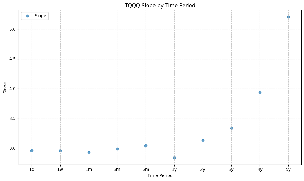
plot_scatter(
    df=rolling_returns_stats,
    x_plot_column="Period",
    y_plot_columns=["Slope"],
    title="TQQQ Slope by Time Period",
    x_label="Time Period",
    x_format="String",
    x_format_decimal_places=0,
    x_tick_spacing=1,
    x_tick_rotation=0,
    y_label="Slope",
    y_format="Decimal",
    y_format_decimal_places=1,
    y_tick_spacing="Auto",
    y_tick_rotation=0,
    plot_OLS_regression_line=False,
    OLS_column=None,
    plot_Ridge_regression_line=False,
    Ridge_column=None,
    plot_RidgeCV_regression_line=False,
    RidgeCV_column=None,
    regression_constant=False,
    grid=True,
    legend=True,
    export_plot=False,
    plot_file_name=None,
)
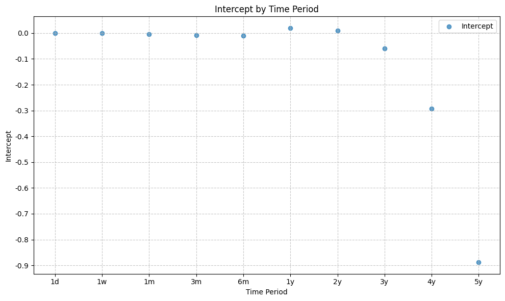
plot_scatter(
    df=rolling_returns_stats,
    x_plot_column="Period",
    y_plot_columns=["Intercept"],
    title="Intercept by Time Period",
    x_label="Time Period",
    x_format="String",
    x_format_decimal_places=0,
    x_tick_spacing=1,
    x_tick_rotation=0,
    y_label="Intercept",
    y_format="Decimal",
    y_format_decimal_places=1,
    y_tick_spacing="Auto",
    y_tick_rotation=0,
    plot_OLS_regression_line=False,
    OLS_column=None,
    plot_Ridge_regression_line=False,
    Ridge_column=None,
    plot_RidgeCV_regression_line=False,
    RidgeCV_column=None,
    regression_constant=False,
    grid=True,
    legend=True,
    export_plot=False,
    plot_file_name=None,
)
display(rolling_returns_stats.set_index("Period"))
| Intercept | Slope | R_Squared | Return Skew | Average Upside Beta | Average Downside Beta | Asymmetry | Return_Deviation_From_3x | |
|---|---|---|---|---|---|---|---|---|
| Period | ||||||||
| 1d | -0.000 | 2.955 | 0.999 | NaN | 2.957 | NaN | NaN | -0.045 |
| 1w | -0.001 | 2.952 | 0.994 | NaN | 2.553 | NaN | NaN | -0.048 |
| 1m | -0.004 | 2.931 | 0.982 | NaN | 2.208 | NaN | NaN | -0.069 |
| 3m | -0.008 | 2.985 | 0.958 | NaN | 1.994 | -inf | inf | -0.015 |
| 6m | -0.010 | 3.040 | 0.916 | -8.728 | 1.478 | 5.417 | -3.939 | 0.040 |
| 1y | 0.019 | 2.837 | 0.880 | NaN | 1.223 | -inf | inf | -0.163 |
| 2y | 0.009 | 3.131 | 0.848 | 36.170 | 1.393 | 12.342 | -10.948 | 0.131 |
| 3y | -0.060 | 3.332 | 0.805 | NaN | -0.088 | -inf | inf | 0.332 |
| 4y | -0.293 | 3.933 | 0.781 | 19.562 | 1.759 | 7.212 | -5.452 | 0.933 |
| 5y | -0.887 | 5.205 | 0.743 | 43.040 | 2.432 | 11.480 | -9.048 | 2.205 |
This is very interesting. Up to 1 year, there is minimal difference between the mean TQQQ 1 year rolling return and the hypothetical 3x leverage, with an R^2 of greater than 0.9.
However, as we extend the time period, we see that
- The “leverage factor” increases significantly, resulting in a deviation from the perfect 3x leverage.
- The intercept also begins to deviate significantly from 0.
The above highlight the impact of volatility magnification over longer time horizons. This phenomenon is happening likely due to the positive returns that QQQ has achieved since 2010 - resulting in TQQQ compounding at a much higher rate than 3x - but it may and likely is not exhibited by other 3x leveraged ETFs that have not had the same positive return profile as QQQ.
With the above results, the next logical question is, when is the opportune time to buy a 3x leveraged ETF like TQQQ? To answer this, we will look a the drawdown levels of TQQQ and the subsequent returns over various time horizons.
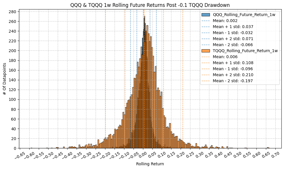
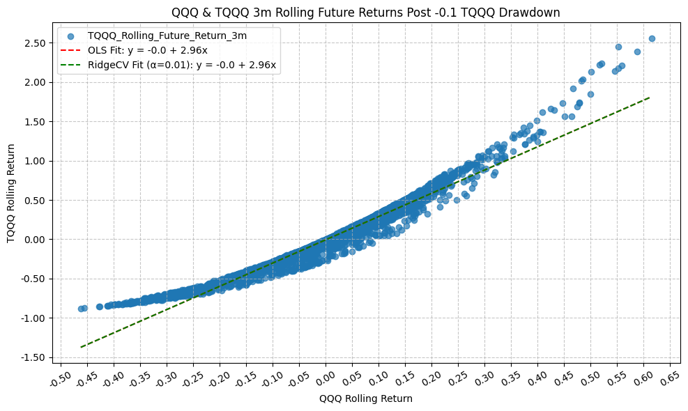
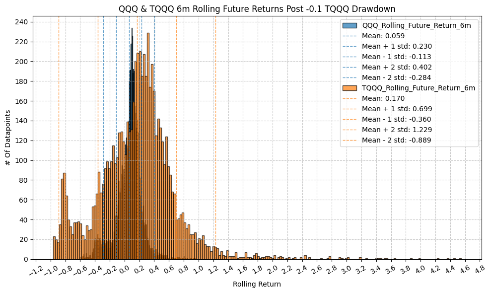
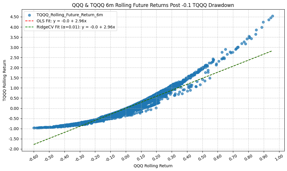
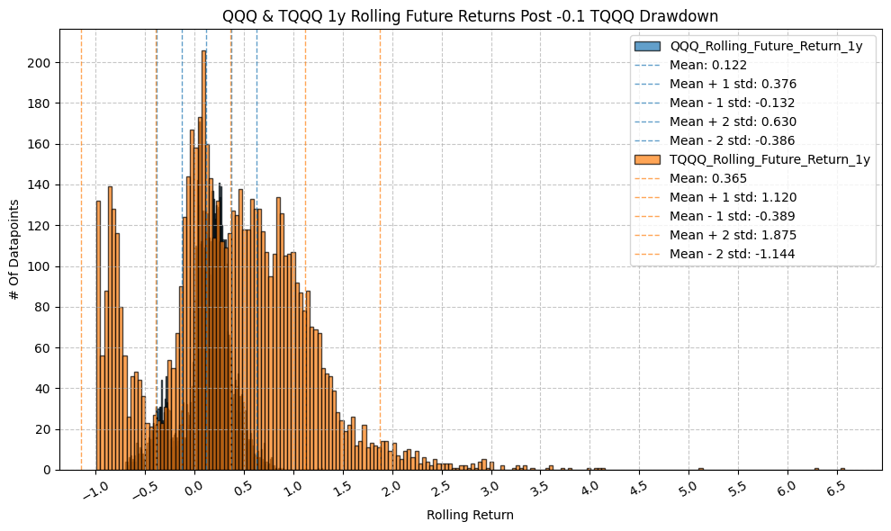
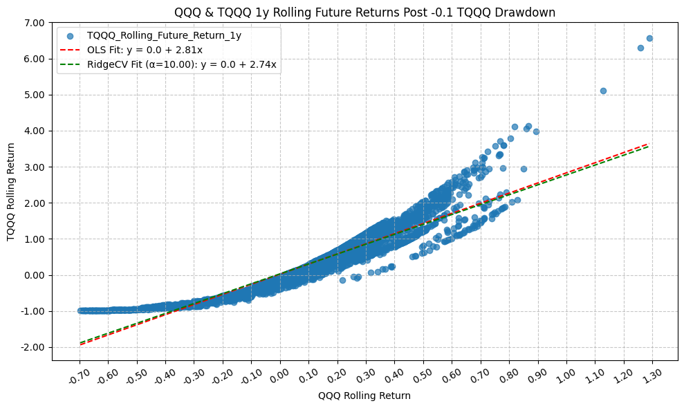
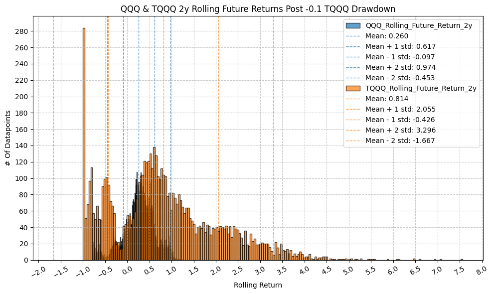
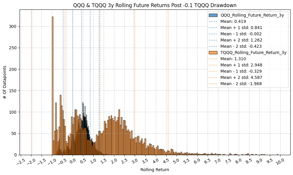
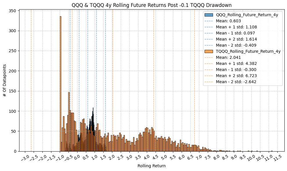
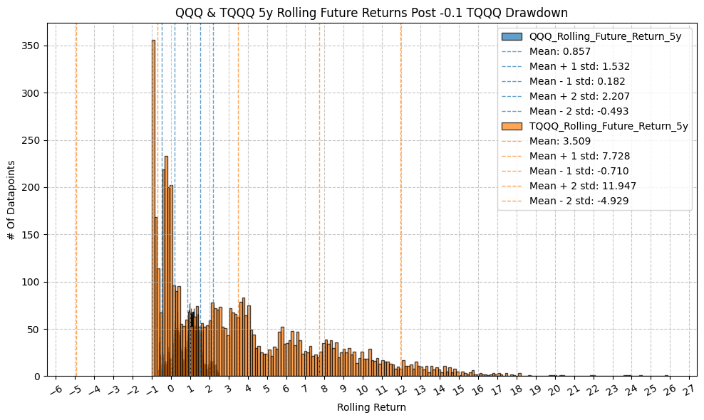
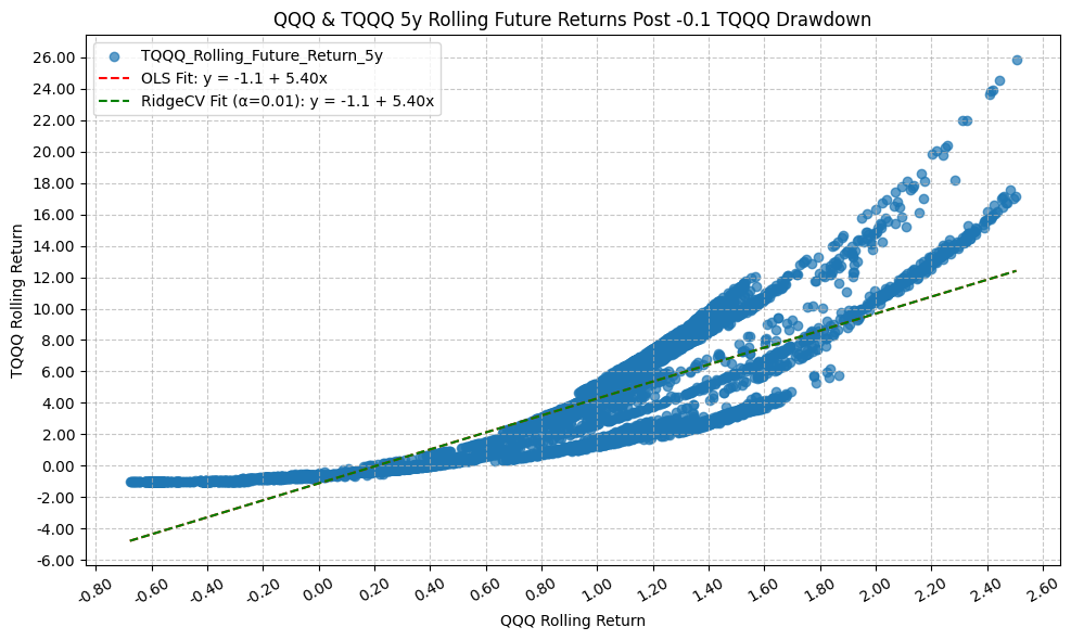
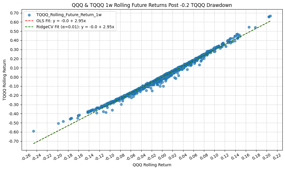
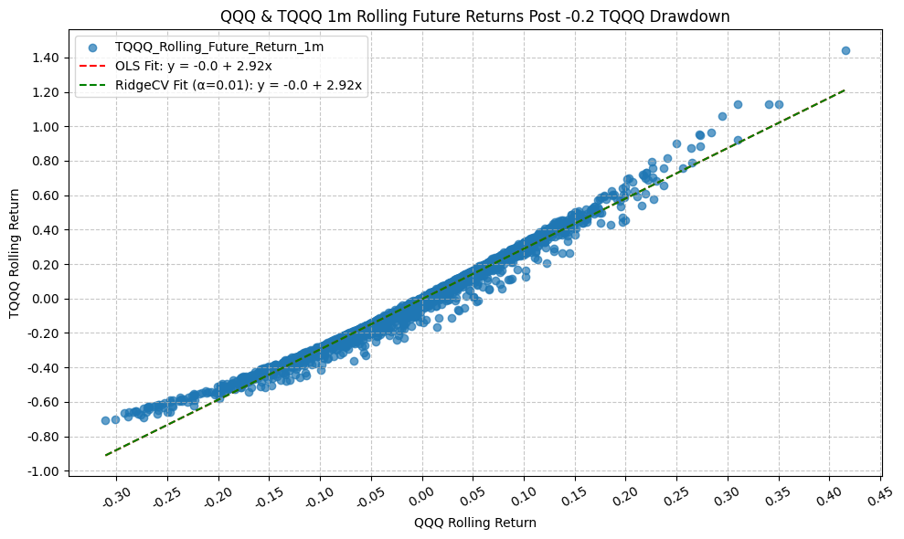
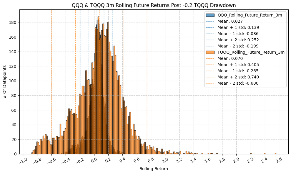
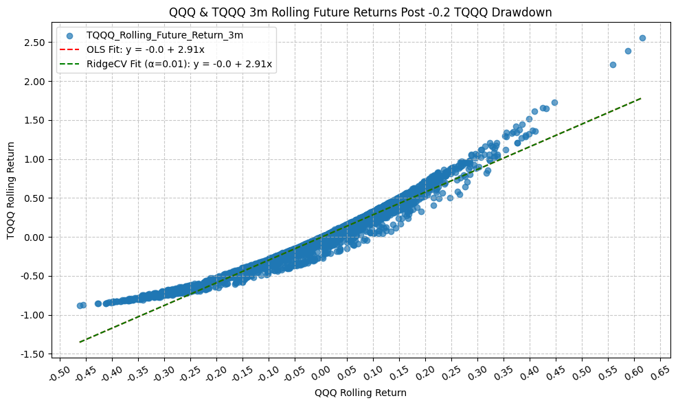
Rolling Returns Following Drawdowns (QQQ & TQQQ) #
We will identify the drawdown levels of TQQQ and then look at the subsequent rolling returns over various time horizons.
# Copy DataFrame
qqq_tqqq_extrap_future = qqq_tqqq_extrap.copy()

# Create a list of drawdown levels to analyze
drawdown_levels = [-0.10, -0.20, -0.30, -0.40, -0.50, -0.60, -0.70, -0.80, -0.90]

# Shift the rolling return columns by the number of days in the rolling window to get the returns following the drawdown
for etf in etfs:
    for period_name, window in rolling_windows.items():
        qqq_tqqq_extrap_future[f"{etf}_Rolling_Future_Return_{period_name}"] = qqq_tqqq_extrap_future[f"{etf}_Rolling_Return_{period_name}"].shift(-window)
Now, we can analyze the future rolling returns following specific drawdown levels:
# Create a dataframe to hold rolling returns stats
rolling_returns_drawdown_stats = pd.DataFrame()

for drawdown in drawdown_levels:

    for period_name, window in rolling_windows.items():

        try:
            plot_histogram(
                df=qqq_tqqq_extrap_future[qqq_tqqq_extrap_future["TQQQ_Drawdown"] <= drawdown],
                plot_columns=[f"QQQ_Rolling_Future_Return_{period_name}", f"TQQQ_Rolling_Future_Return_{period_name}"],
                title=f"QQQ & TQQQ {period_name} Rolling Future Returns Post {drawdown} TQQQ Drawdown",
                x_label="Rolling Return",
                x_tick_spacing="Auto",
                x_tick_rotation=30,
                y_label="# Of Datapoints",
                y_tick_spacing="Auto",
                y_tick_rotation=0,
                grid=True,
                legend=True,
                export_plot=False,
                plot_file_name=None,
            )

            plot_scatter(
                df=qqq_tqqq_extrap_future[qqq_tqqq_extrap_future["TQQQ_Drawdown"] <= drawdown],
                x_plot_column=f"QQQ_Rolling_Future_Return_{period_name}",
                y_plot_columns=[f"TQQQ_Rolling_Future_Return_{period_name}"],
                title=f"QQQ & TQQQ {period_name} Rolling Future Returns Post {drawdown} TQQQ Drawdown",
                x_label="QQQ Rolling Return",
                x_format="Decimal",
                x_format_decimal_places=2,
                x_tick_spacing="Auto",
                x_tick_rotation=30,
                y_label="TQQQ Rolling Return",
                y_format="Decimal",
                y_format_decimal_places=2,
                y_tick_spacing="Auto",
                y_tick_rotation=0,
                plot_OLS_regression_line=True,
                OLS_column=f"TQQQ_Rolling_Future_Return_{period_name}",
                plot_Ridge_regression_line=False,
                Ridge_column=None,
                plot_RidgeCV_regression_line=True,
                RidgeCV_column=f"TQQQ_Rolling_Future_Return_{period_name}",
                regression_constant=True,
                grid=True,
                legend=True,
                export_plot=False,
                plot_file_name=None,
            )

            # Run OLS regression with statsmodels
            model = run_linear_regression(
                df=qqq_tqqq_extrap_future[qqq_tqqq_extrap_future["TQQQ_Drawdown"] <= drawdown],
                x_plot_column=f"QQQ_Rolling_Future_Return_{period_name}",
                y_plot_column=f"TQQQ_Rolling_Future_Return_{period_name}",
                regression_model="OLS-statsmodels",
                regression_constant=True,
            )
            print(model.summary())

            # Filter by drawdown
            drawdown_filter = qqq_tqqq_extrap_future[qqq_tqqq_extrap_future["TQQQ_Drawdown"] <= drawdown]

            # Filter by period, drop rows with missing values
            future_filter = drawdown_filter[[f"TQQQ_Rolling_Future_Return_{period_name}"]].dropna()

            # Find length of future dataframe
            future_length = len(future_filter)

            # Find length of future dataframe where return is positive
            positive_future_length = len(future_filter[future_filter[f"TQQQ_Rolling_Future_Return_{period_name}"] > 0])

            # Calculate percentage of future returns that are positive
            positive_future_percentage = (positive_future_length / future_length) if future_length > 0 else 0

            # Add the regression results to the rolling returns stats dataframe
            intercept = model.params[0]
            # intercept_pvalue = model.pvalues[0]   # p-value for Intercept
            slope = model.params[1]
            # slope_pvalue = model.pvalues[1]       # p-value for Slope
            r_squared = model.rsquared

            rolling_returns_slope_int = pd.DataFrame({
                "Drawdown": drawdown,
                "Period": period_name,
                "Intercept": [intercept],
                # "Intercept_PValue": [intercept_pvalue],
                "Slope": [slope],
                # "Slope_PValue": [slope_pvalue],
                "R_Squared": [r_squared],
                "Positive_Future_Percentage": [positive_future_percentage],
            })

            rolling_returns_drawdown_stats = pd.concat([rolling_returns_drawdown_stats, rolling_returns_slope_int])

        except:
            print(f"Not enough data points for drawdown level {drawdown} and period {period_name} to run regression.")


                                  OLS Regression Results
=========================================================================================
Dep. Variable:     TQQQ_Rolling_Future_Return_1d   R-squared:                       0.999
Model:                                       OLS   Adj. R-squared:                  0.999
Method:                            Least Squares   F-statistic:                 6.829e+06
Date:                           Mon, 23 Mar 2026   Prob (F-statistic):               0.00
Time:                                   21:59:30   Log-Likelihood:                 33568.
No. Observations:                           6653   AIC:                        -6.713e+04
Df Residuals:                               6651   BIC:                        -6.712e+04
Df Model:                                      1
Covariance Type:                       nonrobust
================================================================================================
                                   coef    std err          t      P>|t|      [0.025      0.975]
------------------------------------------------------------------------------------------------
const                        -5.251e-05   1.91e-05     -2.748      0.006      -9e-05    -1.5e-05
QQQ_Rolling_Future_Return_1d     2.9552      0.001   2613.230      0.000       2.953       2.957
==============================================================================
Omnibus:                     9921.143   Durbin-Watson:                   2.565
Prob(Omnibus):                  0.000   Jarque-Bera (JB):         41149977.059
Skew:                          -8.188   Prob(JB):                         0.00
Kurtosis:                     387.936   Cond. No.                         59.2
==============================================================================

Notes:
[1] Standard Errors assume that the covariance matrix of the errors is correctly specified.

                                  OLS Regression Results
=========================================================================================
Dep. Variable:     TQQQ_Rolling_Future_Return_1w   R-squared:                       0.994
Model:                                       OLS   Adj. R-squared:                  0.994
Method:                            Least Squares   F-statistic:                 1.089e+06
Date:                           Mon, 23 Mar 2026   Prob (F-statistic):               0.00
Time:                                   21:59:32   Log-Likelihood:                 22728.
No. Observations:                           6649   AIC:                        -4.545e+04
Df Residuals:                               6647   BIC:                        -4.544e+04
Df Model:                                      1
Covariance Type:                       nonrobust
================================================================================================
                                   coef    std err          t      P>|t|      [0.025      0.975]
------------------------------------------------------------------------------------------------
const                           -0.0008   9.75e-05     -8.250      0.000      -0.001      -0.001
QQQ_Rolling_Future_Return_1w     2.9527      0.003   1043.680      0.000       2.947       2.958
==============================================================================
Omnibus:                     2702.988   Durbin-Watson:                   0.939
Prob(Omnibus):                  0.000   Jarque-Bera (JB):           587592.935
Skew:                          -0.778   Prob(JB):                         0.00
Kurtosis:                      49.028   Cond. No.                         29.1
==============================================================================

Notes:
[1] Standard Errors assume that the covariance matrix of the errors is correctly specified.


                                  OLS Regression Results
=========================================================================================
Dep. Variable:     TQQQ_Rolling_Future_Return_1m   R-squared:                       0.982
Model:                                       OLS   Adj. R-squared:                  0.982
Method:                            Least Squares   F-statistic:                 3.706e+05
Date:                           Mon, 23 Mar 2026   Prob (F-statistic):               0.00
Time:                                   21:59:33   Log-Likelihood:                 14709.
No. Observations:                           6633   AIC:                        -2.941e+04
Df Residuals:                               6631   BIC:                        -2.940e+04
Df Model:                                      1
Covariance Type:                       nonrobust
================================================================================================
                                   coef    std err          t      P>|t|      [0.025      0.975]
------------------------------------------------------------------------------------------------
const                           -0.0035      0.000    -10.565      0.000      -0.004      -0.003
QQQ_Rolling_Future_Return_1m     2.9305      0.005    608.737      0.000       2.921       2.940
==============================================================================
Omnibus:                     1682.131   Durbin-Watson:                   0.312
Prob(Omnibus):                  0.000   Jarque-Bera (JB):            81050.154
Skew:                           0.394   Prob(JB):                         0.00
Kurtosis:                      20.107   Cond. No.                         14.9
==============================================================================

Notes:
[1] Standard Errors assume that the covariance matrix of the errors is correctly specified.

                                  OLS Regression Results
=========================================================================================
Dep. Variable:     TQQQ_Rolling_Future_Return_3m   R-squared:                       0.957
Model:                                       OLS   Adj. R-squared:                  0.957
Method:                            Least Squares   F-statistic:                 1.460e+05
Date:                           Mon, 23 Mar 2026   Prob (F-statistic):               0.00
Time:                                   21:59:35   Log-Likelihood:                 7955.3
No. Observations:                           6591   AIC:                        -1.591e+04
Df Residuals:                               6589   BIC:                        -1.589e+04
Df Model:                                      1
Covariance Type:                       nonrobust
================================================================================================
                                   coef    std err          t      P>|t|      [0.025      0.975]
------------------------------------------------------------------------------------------------
const                           -0.0076      0.001     -8.295      0.000      -0.009      -0.006
QQQ_Rolling_Future_Return_3m     2.9584      0.008    382.045      0.000       2.943       2.974
==============================================================================
Omnibus:                     3406.252   Durbin-Watson:                   0.113
Prob(Omnibus):                  0.000   Jarque-Bera (JB):            86494.126
Skew:                           1.943   Prob(JB):                         0.00
Kurtosis:                      20.316   Cond. No.                         8.69
==============================================================================

Notes:
[1] Standard Errors assume that the covariance matrix of the errors is correctly specified.
                                  OLS Regression Results
=========================================================================================
Dep. Variable:     TQQQ_Rolling_Future_Return_6m   R-squared:                       0.921
Model:                                       OLS   Adj. R-squared:                  0.921
Method:                            Least Squares   F-statistic:                 7.570e+04
Date:                           Mon, 23 Mar 2026   Prob (F-statistic):               0.00
Time:                                   21:59:37   Log-Likelihood:                 3158.3
No. Observations:                           6528   AIC:                            -6313.
Df Residuals:                               6526   BIC:                            -6299.
Df Model:                                      1
Covariance Type:                       nonrobust
================================================================================================
                                   coef    std err          t      P>|t|      [0.025      0.975]
------------------------------------------------------------------------------------------------
const                           -0.0042      0.002     -2.170      0.030      -0.008      -0.000
QQQ_Rolling_Future_Return_6m     2.9628      0.011    275.145      0.000       2.942       2.984
==============================================================================
Omnibus:                     4159.114   Durbin-Watson:                   0.065
Prob(Omnibus):                  0.000   Jarque-Bera (JB):           100812.187
Skew:                           2.648   Prob(JB):                         0.00
Kurtosis:                      21.509   Cond. No.                         5.85
==============================================================================

Notes:
[1] Standard Errors assume that the covariance matrix of the errors is correctly specified.
                                  OLS Regression Results
=========================================================================================
Dep. Variable:     TQQQ_Rolling_Future_Return_1y   R-squared:                       0.893
Model:                                       OLS   Adj. R-squared:                  0.893
Method:                            Least Squares   F-statistic:                 5.327e+04
Date:                           Mon, 23 Mar 2026   Prob (F-statistic):               0.00
Time:                                   21:59:38   Log-Likelihood:                -135.02
No. Observations:                           6402   AIC:                             274.0
Df Residuals:                               6400   BIC:                             287.6
Df Model:                                      1
Covariance Type:                       nonrobust
================================================================================================
                                   coef    std err          t      P>|t|      [0.025      0.975]
------------------------------------------------------------------------------------------------
const                            0.0227      0.003      6.620      0.000       0.016       0.029
QQQ_Rolling_Future_Return_1y     2.8086      0.012    230.806      0.000       2.785       2.832
==============================================================================
Omnibus:                     2635.410   Durbin-Watson:                   0.052
Prob(Omnibus):                  0.000   Jarque-Bera (JB):            29285.399
Skew:                           1.658   Prob(JB):                         0.00
Kurtosis:                      12.939   Cond. No.                         4.00
==============================================================================

Notes:
[1] Standard Errors assume that the covariance matrix of the errors is correctly specified.

                                  OLS Regression Results
=========================================================================================
Dep. Variable:     TQQQ_Rolling_Future_Return_2y   R-squared:                       0.848
Model:                                       OLS   Adj. R-squared:                  0.848
Method:                            Least Squares   F-statistic:                 3.424e+04
Date:                           Mon, 23 Mar 2026   Prob (F-statistic):               0.00
Time:                                   21:59:40   Log-Likelihood:                -4264.9
No. Observations:                           6150   AIC:                             8534.
Df Residuals:                               6148   BIC:                             8547.
Df Model:                                      1
Covariance Type:                       nonrobust
================================================================================================
                                   coef    std err          t      P>|t|      [0.025      0.975]
------------------------------------------------------------------------------------------------
const                           -0.0192      0.008     -2.513      0.012      -0.034      -0.004
QQQ_Rolling_Future_Return_2y     3.2011      0.017    185.033      0.000       3.167       3.235
==============================================================================
Omnibus:                     1671.115   Durbin-Watson:                   0.019
Prob(Omnibus):                  0.000   Jarque-Bera (JB):             4642.964
Skew:                           1.436   Prob(JB):                         0.00
Kurtosis:                       6.142   Cond. No.                         3.02
==============================================================================

Notes:
[1] Standard Errors assume that the covariance matrix of the errors is correctly specified.
                                  OLS Regression Results
=========================================================================================
Dep. Variable:     TQQQ_Rolling_Future_Return_3y   R-squared:                       0.811
Model:                                       OLS   Adj. R-squared:                  0.811
Method:                            Least Squares   F-statistic:                 2.527e+04
Date:                           Mon, 23 Mar 2026   Prob (F-statistic):               0.00
Time:                                   21:59:42   Log-Likelihood:                -6371.3
No. Observations:                           5898   AIC:                         1.275e+04
Df Residuals:                               5896   BIC:                         1.276e+04
Df Model:                                      1
Covariance Type:                       nonrobust
================================================================================================
                                   coef    std err          t      P>|t|      [0.025      0.975]
------------------------------------------------------------------------------------------------
const                           -0.1589      0.013    -12.137      0.000      -0.185      -0.133
QQQ_Rolling_Future_Return_3y     3.5019      0.022    158.976      0.000       3.459       3.545
==============================================================================
Omnibus:                      871.703   Durbin-Watson:                   0.015
Prob(Omnibus):                  0.000   Jarque-Bera (JB):             1536.806
Skew:                           0.961   Prob(JB):                         0.00
Kurtosis:                       4.601   Cond. No.                         2.86
==============================================================================

Notes:
[1] Standard Errors assume that the covariance matrix of the errors is correctly specified.

                                  OLS Regression Results
=========================================================================================
Dep. Variable:     TQQQ_Rolling_Future_Return_4y   R-squared:                       0.783
Model:                                       OLS   Adj. R-squared:                  0.783
Method:                            Least Squares   F-statistic:                 2.034e+04
Date:                           Mon, 23 Mar 2026   Prob (F-statistic):               0.00
Time:                                   21:59:44   Log-Likelihood:                -8503.0
No. Observations:                           5646   AIC:                         1.701e+04
Df Residuals:                               5644   BIC:                         1.702e+04
Df Model:                                      1
Covariance Type:                       nonrobust
================================================================================================
                                   coef    std err          t      P>|t|      [0.025      0.975]
------------------------------------------------------------------------------------------------
const                           -0.4276      0.023    -18.927      0.000      -0.472      -0.383
QQQ_Rolling_Future_Return_4y     4.0962      0.029    142.630      0.000       4.040       4.153
==============================================================================
Omnibus:                      127.164   Durbin-Watson:                   0.010
Prob(Omnibus):                  0.000   Jarque-Bera (JB):               79.194
Skew:                           0.148   Prob(JB):                     6.36e-18
Kurtosis:                       2.501   Cond. No.                         2.85
==============================================================================

Notes:
[1] Standard Errors assume that the covariance matrix of the errors is correctly specified.
                                  OLS Regression Results
=========================================================================================
Dep. Variable:     TQQQ_Rolling_Future_Return_5y   R-squared:                       0.745
Model:                                       OLS   Adj. R-squared:                  0.745
Method:                            Least Squares   F-statistic:                 1.577e+04
Date:                           Mon, 23 Mar 2026   Prob (F-statistic):               0.00
Time:                                   21:59:46   Log-Likelihood:                -11731.
No. Observations:                           5394   AIC:                         2.347e+04
Df Residuals:                               5392   BIC:                         2.348e+04
Df Model:                                      1
Covariance Type:                       nonrobust
================================================================================================
                                   coef    std err          t      P>|t|      [0.025      0.975]
------------------------------------------------------------------------------------------------
const                           -1.1160      0.047    -23.806      0.000      -1.208      -1.024
QQQ_Rolling_Future_Return_5y     5.3968      0.043    125.578      0.000       5.313       5.481
==============================================================================
Omnibus:                      276.642   Durbin-Watson:                   0.009
Prob(Omnibus):                  0.000   Jarque-Bera (JB):              406.454
Skew:                           0.460   Prob(JB):                     5.49e-89
Kurtosis:                       3.980   Cond. No.                         2.90
==============================================================================

Notes:
[1] Standard Errors assume that the covariance matrix of the errors is correctly specified.


                                  OLS Regression Results
=========================================================================================
Dep. Variable:     TQQQ_Rolling_Future_Return_1d   R-squared:                       0.999
Model:                                       OLS   Adj. R-squared:                  0.999
Method:                            Least Squares   F-statistic:                 6.607e+06
Date:                           Mon, 23 Mar 2026   Prob (F-statistic):               0.00
Time:                                   21:59:47   Log-Likelihood:                 33141.
No. Observations:                           6576   AIC:                        -6.628e+04
Df Residuals:                               6574   BIC:                        -6.626e+04
Df Model:                                      1
Covariance Type:                       nonrobust
================================================================================================
                                   coef    std err          t      P>|t|      [0.025      0.975]
------------------------------------------------------------------------------------------------
const                        -5.312e-05   1.93e-05     -2.748      0.006    -9.1e-05   -1.52e-05
QQQ_Rolling_Future_Return_1d     2.9552      0.001   2570.336      0.000       2.953       2.957
==============================================================================
Omnibus:                     9776.502   Durbin-Watson:                   2.565
Prob(Omnibus):                  0.000   Jarque-Bera (JB):         39728976.844
Skew:                          -8.139   Prob(JB):                         0.00
Kurtosis:                     383.436   Cond. No.                         59.5
==============================================================================

Notes:
[1] Standard Errors assume that the covariance matrix of the errors is correctly specified.

                                  OLS Regression Results
=========================================================================================
Dep. Variable:     TQQQ_Rolling_Future_Return_1w   R-squared:                       0.994
Model:                                       OLS   Adj. R-squared:                  0.994
Method:                            Least Squares   F-statistic:                 1.070e+06
Date:                           Mon, 23 Mar 2026   Prob (F-statistic):               0.00
Time:                                   21:59:49   Log-Likelihood:                 22472.
No. Observations:                           6572   AIC:                        -4.494e+04
Df Residuals:                               6570   BIC:                        -4.493e+04
Df Model:                                      1
Covariance Type:                       nonrobust
================================================================================================
                                   coef    std err          t      P>|t|      [0.025      0.975]
------------------------------------------------------------------------------------------------
const                           -0.0008   9.79e-05     -8.045      0.000      -0.001      -0.001
QQQ_Rolling_Future_Return_1w     2.9518      0.003   1034.395      0.000       2.946       2.957
==============================================================================
Omnibus:                     2706.760   Durbin-Watson:                   0.933
Prob(Omnibus):                  0.000   Jarque-Bera (JB):           596172.137
Skew:                          -0.802   Prob(JB):                         0.00
Kurtosis:                      49.632   Cond. No.                         29.2
==============================================================================

Notes:
[1] Standard Errors assume that the covariance matrix of the errors is correctly specified.

                                  OLS Regression Results
=========================================================================================
Dep. Variable:     TQQQ_Rolling_Future_Return_1m   R-squared:                       0.983
Model:                                       OLS   Adj. R-squared:                  0.983
Method:                            Least Squares   F-statistic:                 3.706e+05
Date:                           Mon, 23 Mar 2026   Prob (F-statistic):               0.00
Time:                                   21:59:50   Log-Likelihood:                 14666.
No. Observations:                           6556   AIC:                        -2.933e+04
Df Residuals:                               6554   BIC:                        -2.931e+04
Df Model:                                      1
Covariance Type:                       nonrobust
================================================================================================
                                   coef    std err          t      P>|t|      [0.025      0.975]
------------------------------------------------------------------------------------------------
const                           -0.0035      0.000    -10.838      0.000      -0.004      -0.003
QQQ_Rolling_Future_Return_1m     2.9225      0.005    608.738      0.000       2.913       2.932
==============================================================================
Omnibus:                     1537.890   Durbin-Watson:                   0.317
Prob(Omnibus):                  0.000   Jarque-Bera (JB):            81206.359
Skew:                           0.161   Prob(JB):                         0.00
Kurtosis:                      20.239   Cond. No.                         15.0
==============================================================================

Notes:
[1] Standard Errors assume that the covariance matrix of the errors is correctly specified.
                                  OLS Regression Results
=========================================================================================
Dep. Variable:     TQQQ_Rolling_Future_Return_3m   R-squared:                       0.960
Model:                                       OLS   Adj. R-squared:                  0.960
Method:                            Least Squares   F-statistic:                 1.545e+05
Date:                           Mon, 23 Mar 2026   Prob (F-statistic):               0.00
Time:                                   21:59:52   Log-Likelihood:                 8329.3
No. Observations:                           6514   AIC:                        -1.665e+04
Df Residuals:                               6512   BIC:                        -1.664e+04
Df Model:                                      1
Covariance Type:                       nonrobust
================================================================================================
                                   coef    std err          t      P>|t|      [0.025      0.975]
------------------------------------------------------------------------------------------------
const                           -0.0070      0.001     -8.214      0.000      -0.009      -0.005
QQQ_Rolling_Future_Return_3m     2.9105      0.007    393.118      0.000       2.896       2.925
==============================================================================
Omnibus:                     2149.722   Durbin-Watson:                   0.136
Prob(Omnibus):                  0.000   Jarque-Bera (JB):            38861.452
Skew:                           1.110   Prob(JB):                         0.00
Kurtosis:                      14.758   Cond. No.                         8.88
==============================================================================

Notes:
[1] Standard Errors assume that the covariance matrix of the errors is correctly specified.


                                  OLS Regression Results
=========================================================================================
Dep. Variable:     TQQQ_Rolling_Future_Return_6m   R-squared:                       0.926
Model:                                       OLS   Adj. R-squared:                  0.926
Method:                            Least Squares   F-statistic:                 8.107e+04
Date:                           Mon, 23 Mar 2026   Prob (F-statistic):               0.00
Time:                                   21:59:54   Log-Likelihood:                 3783.3
No. Observations:                           6451   AIC:                            -7563.
Df Residuals:                               6449   BIC:                            -7549.
Df Model:                                      1
Covariance Type:                       nonrobust
================================================================================================
                                   coef    std err          t      P>|t|      [0.025      0.975]
------------------------------------------------------------------------------------------------
const                           -0.0016      0.002     -0.902      0.367      -0.005       0.002
QQQ_Rolling_Future_Return_6m     2.8745      0.010    284.728      0.000       2.855       2.894
==============================================================================
Omnibus:                     3187.487   Durbin-Watson:                   0.077
Prob(Omnibus):                  0.000   Jarque-Bera (JB):            49858.855
Skew:                           1.979   Prob(JB):                         0.00
Kurtosis:                      16.032   Cond. No.                         6.04
==============================================================================

Notes:
[1] Standard Errors assume that the covariance matrix of the errors is correctly specified.
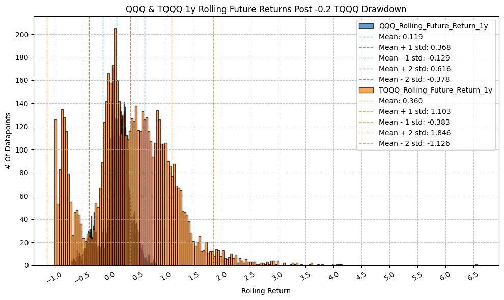
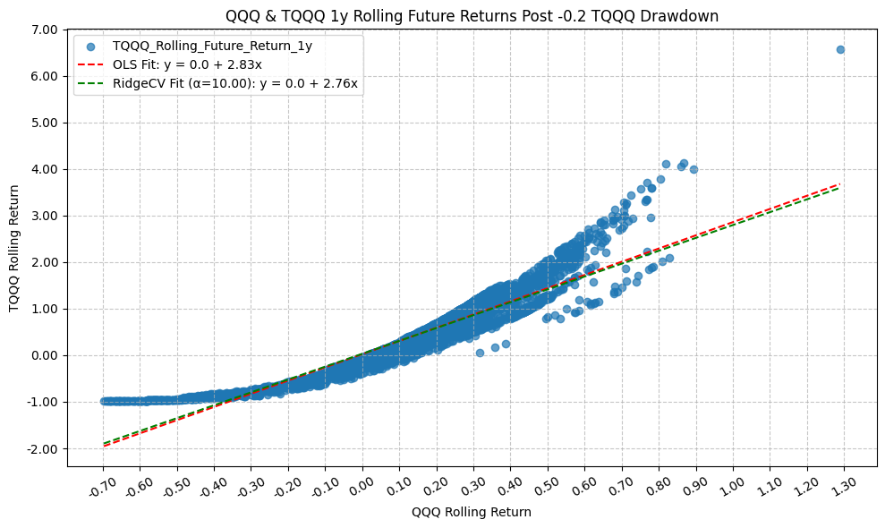
                                  OLS Regression Results
=========================================================================================
Dep. Variable:     TQQQ_Rolling_Future_Return_1y   R-squared:                       0.898
Model:                                       OLS   Adj. R-squared:                  0.898
Method:                            Least Squares   F-statistic:                 5.552e+04
Date:                           Mon, 23 Mar 2026   Prob (F-statistic):               0.00
Time:                                   21:59:55   Log-Likelihood:                 116.33
No. Observations:                           6325   AIC:                            -228.7
Df Residuals:                               6323   BIC:                            -215.2
Df Model:                                      1
Covariance Type:                       nonrobust
================================================================================================
                                   coef    std err          t      P>|t|      [0.025      0.975]
------------------------------------------------------------------------------------------------
const                            0.0225      0.003      6.800      0.000       0.016       0.029
QQQ_Rolling_Future_Return_1y     2.8341      0.012    235.629      0.000       2.811       2.858
==============================================================================
Omnibus:                     2426.355   Durbin-Watson:                   0.068
Prob(Omnibus):                  0.000   Jarque-Bera (JB):            19481.948
Skew:                           1.622   Prob(JB):                         0.00
Kurtosis:                      10.963   Cond. No.                         4.09
==============================================================================

Notes:
[1] Standard Errors assume that the covariance matrix of the errors is correctly specified.
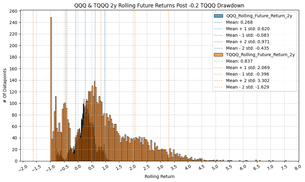

                                  OLS Regression Results
=========================================================================================
Dep. Variable:     TQQQ_Rolling_Future_Return_2y   R-squared:                       0.847
Model:                                       OLS   Adj. R-squared:                  0.847
Method:                            Least Squares   F-statistic:                 3.363e+04
Date:                           Mon, 23 Mar 2026   Prob (F-statistic):               0.00
Time:                                   21:59:57   Log-Likelihood:                -4185.9
No. Observations:                           6073   AIC:                             8376.
Df Residuals:                               6071   BIC:                             8389.
Df Model:                                      1
Covariance Type:                       nonrobust
================================================================================================
                                   coef    std err          t      P>|t|      [0.025      0.975]
------------------------------------------------------------------------------------------------
const                           -0.0292      0.008     -3.748      0.000      -0.044      -0.014
QQQ_Rolling_Future_Return_2y     3.2273      0.018    183.386      0.000       3.193       3.262
==============================================================================
Omnibus:                     1696.489   Durbin-Watson:                   0.019
Prob(Omnibus):                  0.000   Jarque-Bera (JB):             4868.815
Skew:                           1.463   Prob(JB):                         0.00
Kurtosis:                       6.269   Cond. No.                         3.08
==============================================================================

Notes:
[1] Standard Errors assume that the covariance matrix of the errors is correctly specified.
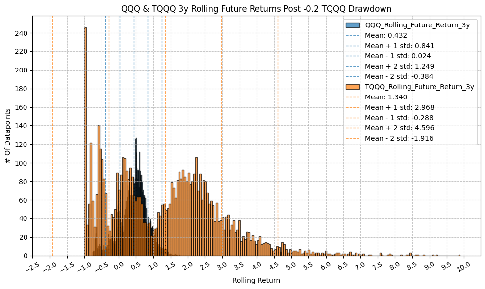
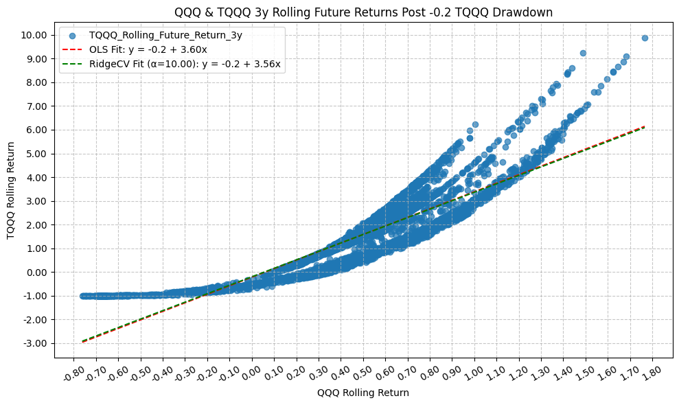
                                  OLS Regression Results
=========================================================================================
Dep. Variable:     TQQQ_Rolling_Future_Return_3y   R-squared:                       0.814
Model:                                       OLS   Adj. R-squared:                  0.814
Method:                            Least Squares   F-statistic:                 2.553e+04
Date:                           Mon, 23 Mar 2026   Prob (F-statistic):               0.00
Time:                                   21:59:59   Log-Likelihood:                -6195.0
No. Observations:                           5821   AIC:                         1.239e+04
Df Residuals:                               5819   BIC:                         1.241e+04
Df Model:                                      1
Covariance Type:                       nonrobust
================================================================================================
                                   coef    std err          t      P>|t|      [0.025      0.975]
------------------------------------------------------------------------------------------------
const                           -0.2169      0.013    -16.188      0.000      -0.243      -0.191
QQQ_Rolling_Future_Return_3y     3.6000      0.023    159.772      0.000       3.556       3.644
==============================================================================
Omnibus:                      877.246   Durbin-Watson:                   0.015
Prob(Omnibus):                  0.000   Jarque-Bera (JB):             1578.522
Skew:                           0.967   Prob(JB):                         0.00
Kurtosis:                       4.663   Cond. No.                         2.98
==============================================================================

Notes:
[1] Standard Errors assume that the covariance matrix of the errors is correctly specified.
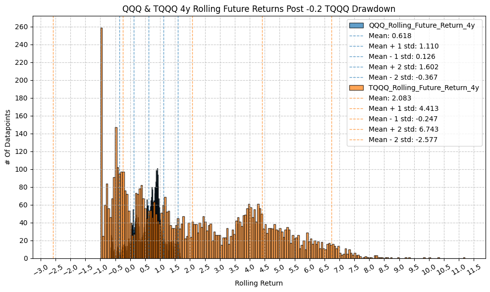
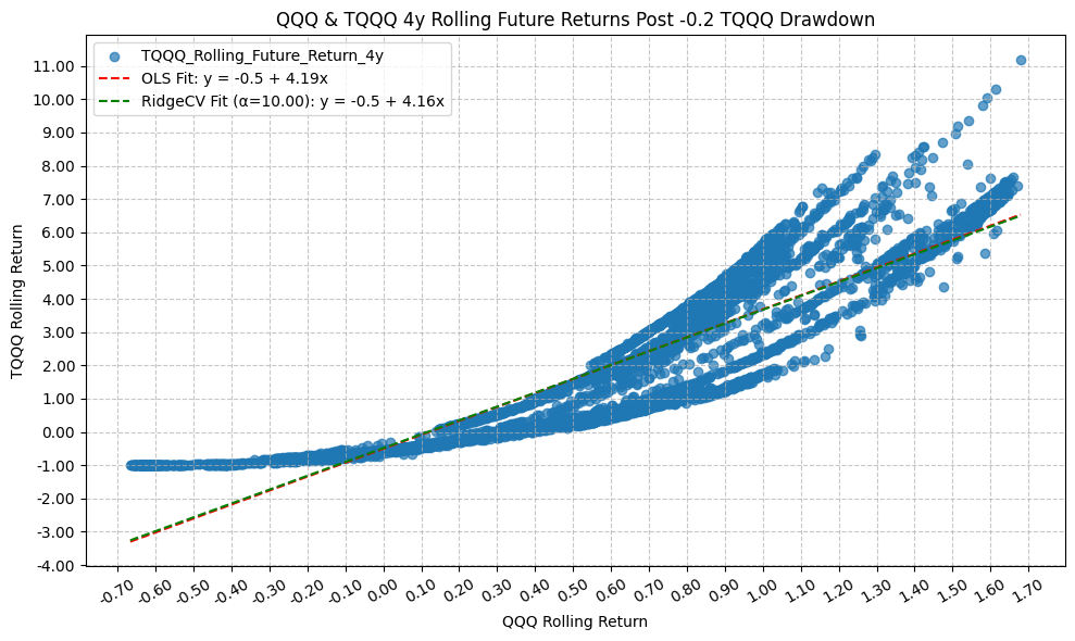
                                  OLS Regression Results
=========================================================================================
Dep. Variable:     TQQQ_Rolling_Future_Return_4y   R-squared:                       0.784
Model:                                       OLS   Adj. R-squared:                  0.784
Method:                            Least Squares   F-statistic:                 2.020e+04
Date:                           Mon, 23 Mar 2026   Prob (F-statistic):               0.00
Time:                                   22:00:00   Log-Likelihood:                -8345.7
No. Observations:                           5569   AIC:                         1.670e+04
Df Residuals:                               5567   BIC:                         1.671e+04
Df Model:                                      1
Covariance Type:                       nonrobust
================================================================================================
                                   coef    std err          t      P>|t|      [0.025      0.975]
------------------------------------------------------------------------------------------------
const                           -0.5067      0.023    -21.753      0.000      -0.552      -0.461
QQQ_Rolling_Future_Return_4y     4.1913      0.029    142.118      0.000       4.134       4.249
==============================================================================
Omnibus:                       90.780   Durbin-Watson:                   0.010
Prob(Omnibus):                  0.000   Jarque-Bera (JB):               63.985
Skew:                           0.153   Prob(JB):                     1.28e-14
Kurtosis:                       2.573   Cond. No.                         2.96
==============================================================================

Notes:
[1] Standard Errors assume that the covariance matrix of the errors is correctly specified.
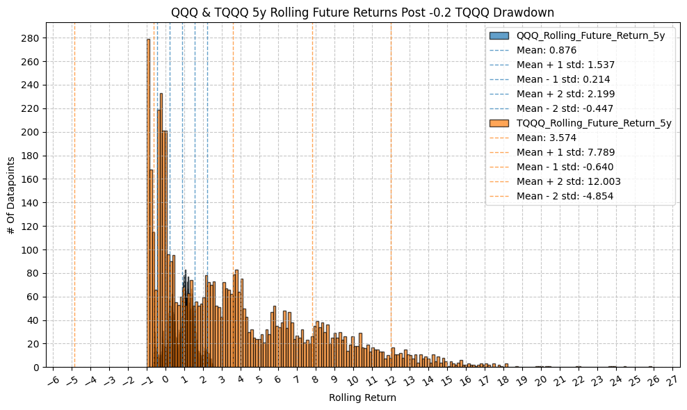

                                  OLS Regression Results
=========================================================================================
Dep. Variable:     TQQQ_Rolling_Future_Return_5y   R-squared:                       0.746
Model:                                       OLS   Adj. R-squared:                  0.746
Method:                            Least Squares   F-statistic:                 1.565e+04
Date:                           Mon, 23 Mar 2026   Prob (F-statistic):               0.00
Time:                                   22:00:02   Log-Likelihood:                -11544.
No. Observations:                           5317   AIC:                         2.309e+04
Df Residuals:                               5315   BIC:                         2.311e+04
Df Model:                                      1
Covariance Type:                       nonrobust
================================================================================================
                                   coef    std err          t      P>|t|      [0.025      0.975]
------------------------------------------------------------------------------------------------
const                           -1.2461      0.048    -25.807      0.000      -1.341      -1.151
QQQ_Rolling_Future_Return_5y     5.5050      0.044    125.105      0.000       5.419       5.591
==============================================================================
Omnibus:                      257.259   Durbin-Watson:                   0.009
Prob(Omnibus):                  0.000   Jarque-Bera (JB):              381.231
Skew:                           0.438   Prob(JB):                     1.65e-83
Kurtosis:                       3.976   Cond. No.                         3.00
==============================================================================

Notes:
[1] Standard Errors assume that the covariance matrix of the errors is correctly specified.
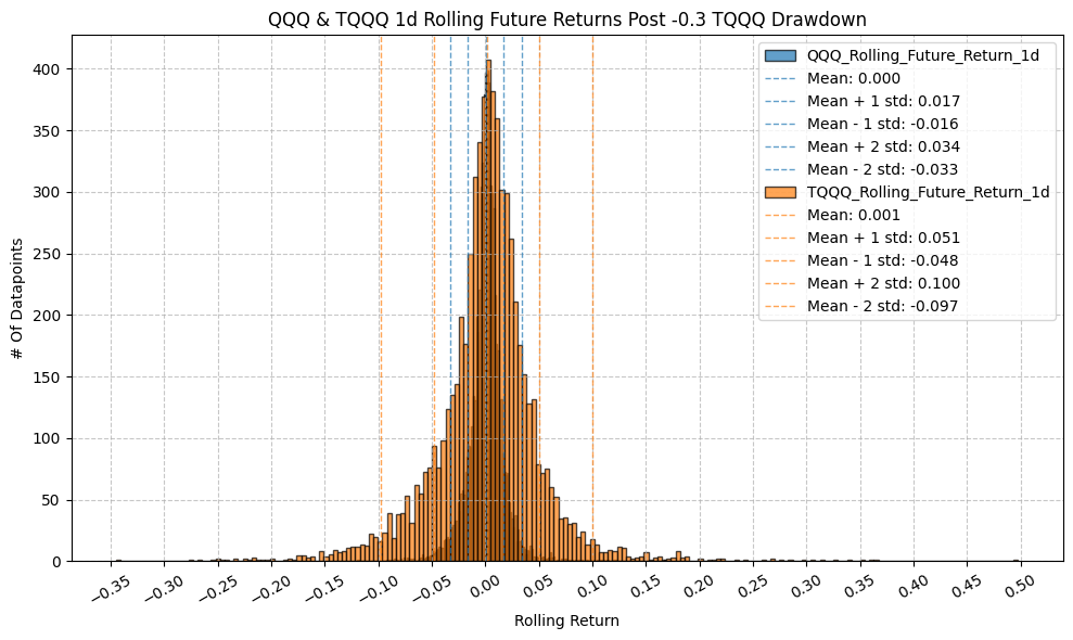
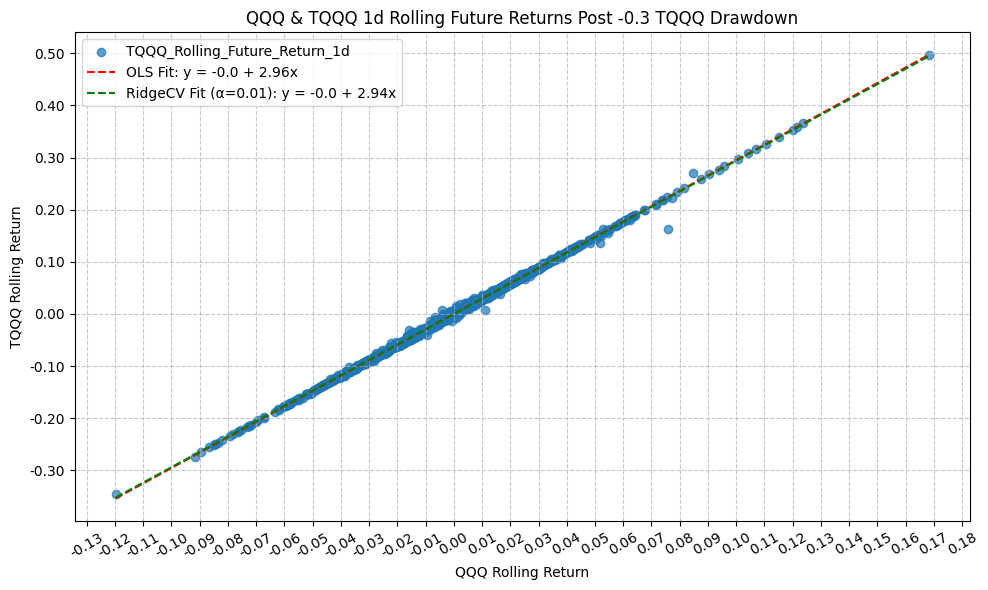
                                  OLS Regression Results
=========================================================================================
Dep. Variable:     TQQQ_Rolling_Future_Return_1d   R-squared:                       0.999
Model:                                       OLS   Adj. R-squared:                  0.999
Method:                            Least Squares   F-statistic:                 6.438e+06
Date:                           Mon, 23 Mar 2026   Prob (F-statistic):               0.00
Time:                                   22:00:04   Log-Likelihood:                 32920.
No. Observations:                           6536   AIC:                        -6.584e+04
Df Residuals:                               6534   BIC:                        -6.582e+04
Df Model:                                      1
Covariance Type:                       nonrobust
================================================================================================
                                   coef    std err          t      P>|t|      [0.025      0.975]
------------------------------------------------------------------------------------------------
const                        -5.345e-05   1.95e-05     -2.748      0.006   -9.16e-05   -1.53e-05
QQQ_Rolling_Future_Return_1d     2.9552      0.001   2537.269      0.000       2.953       2.957
==============================================================================
Omnibus:                     9701.531   Durbin-Watson:                   2.565
Prob(Omnibus):                  0.000   Jarque-Bera (JB):         39004118.756
Skew:                          -8.113   Prob(JB):                         0.00
Kurtosis:                     381.099   Cond. No.                         59.9
==============================================================================

Notes:
[1] Standard Errors assume that the covariance matrix of the errors is correctly specified.
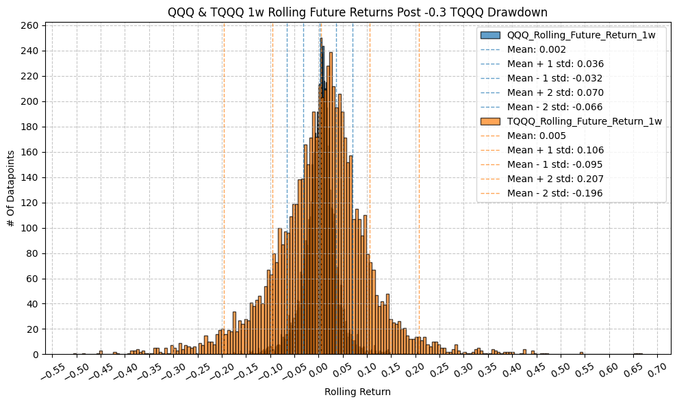

                                  OLS Regression Results
=========================================================================================
Dep. Variable:     TQQQ_Rolling_Future_Return_1w   R-squared:                       0.994
Model:                                       OLS   Adj. R-squared:                  0.994
Method:                            Least Squares   F-statistic:                 1.120e+06
Date:                           Mon, 23 Mar 2026   Prob (F-statistic):               0.00
Time:                                   22:00:05   Log-Likelihood:                 22539.
No. Observations:                           6532   AIC:                        -4.507e+04
Df Residuals:                               6530   BIC:                        -4.506e+04
Df Model:                                      1
Covariance Type:                       nonrobust
================================================================================================
                                   coef    std err          t      P>|t|      [0.025      0.975]
------------------------------------------------------------------------------------------------
const                           -0.0008   9.52e-05     -8.363      0.000      -0.001      -0.001
QQQ_Rolling_Future_Return_1w     2.9553      0.003   1058.242      0.000       2.950       2.961
==============================================================================
Omnibus:                     3465.972   Durbin-Watson:                   0.902
Prob(Omnibus):                  0.000   Jarque-Bera (JB):           389191.684
Skew:                          -1.579   Prob(JB):                         0.00
Kurtosis:                      40.683   Cond. No.                         29.4
==============================================================================

Notes:
[1] Standard Errors assume that the covariance matrix of the errors is correctly specified.


                                  OLS Regression Results
=========================================================================================
Dep. Variable:     TQQQ_Rolling_Future_Return_1m   R-squared:                       0.983
Model:                                       OLS   Adj. R-squared:                  0.983
Method:                            Least Squares   F-statistic:                 3.677e+05
Date:                           Mon, 23 Mar 2026   Prob (F-statistic):               0.00
Time:                                   22:00:07   Log-Likelihood:                 14636.
No. Observations:                           6516   AIC:                        -2.927e+04
Df Residuals:                               6514   BIC:                        -2.925e+04
Df Model:                                      1
Covariance Type:                       nonrobust
================================================================================================
                                   coef    std err          t      P>|t|      [0.025      0.975]
------------------------------------------------------------------------------------------------
const                           -0.0035      0.000    -11.070      0.000      -0.004      -0.003
QQQ_Rolling_Future_Return_1m     2.9177      0.005    606.418      0.000       2.908       2.927
==============================================================================
Omnibus:                     1513.769   Durbin-Watson:                   0.308
Prob(Omnibus):                  0.000   Jarque-Bera (JB):            82043.239
Skew:                           0.084   Prob(JB):                         0.00
Kurtosis:                      20.383   Cond. No.                         15.2
==============================================================================

Notes:
[1] Standard Errors assume that the covariance matrix of the errors is correctly specified.


                                  OLS Regression Results
=========================================================================================
Dep. Variable:     TQQQ_Rolling_Future_Return_3m   R-squared:                       0.961
Model:                                       OLS   Adj. R-squared:                  0.961
Method:                            Least Squares   F-statistic:                 1.586e+05
Date:                           Mon, 23 Mar 2026   Prob (F-statistic):               0.00
Time:                                   22:00:09   Log-Likelihood:                 8465.8
No. Observations:                           6474   AIC:                        -1.693e+04
Df Residuals:                               6472   BIC:                        -1.691e+04
Df Model:                                      1
Covariance Type:                       nonrobust
================================================================================================
                                   coef    std err          t      P>|t|      [0.025      0.975]
------------------------------------------------------------------------------------------------
const                           -0.0067      0.001     -8.081      0.000      -0.008      -0.005
QQQ_Rolling_Future_Return_3m     2.8944      0.007    398.234      0.000       2.880       2.909
==============================================================================
Omnibus:                     1349.017   Durbin-Watson:                   0.103
Prob(Omnibus):                  0.000   Jarque-Bera (JB):            15307.847
Skew:                           0.668   Prob(JB):                         0.00
Kurtosis:                      10.414   Cond. No.                         8.94
==============================================================================

Notes:
[1] Standard Errors assume that the covariance matrix of the errors is correctly specified.
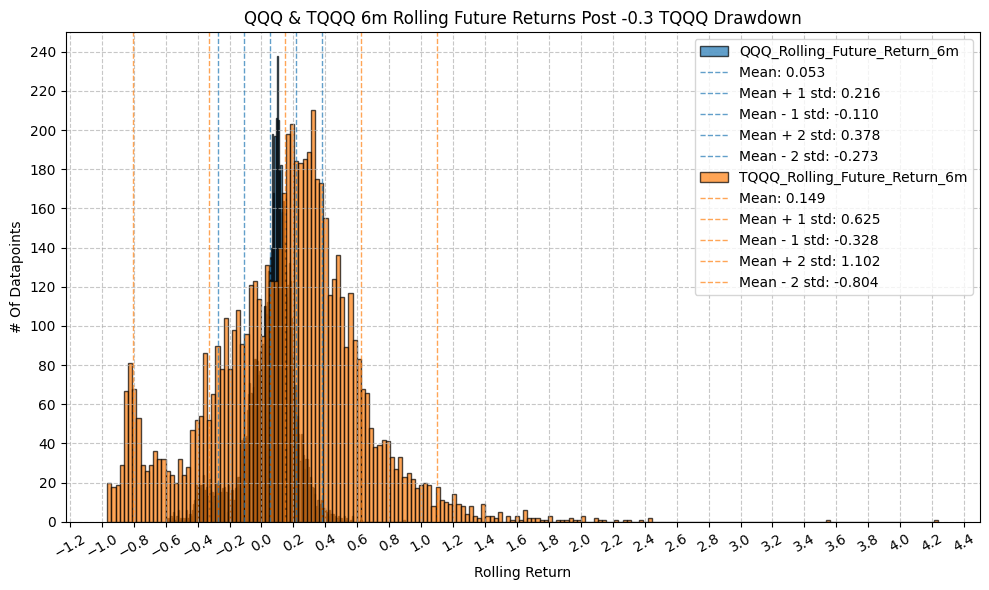
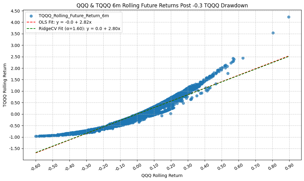
                                  OLS Regression Results
=========================================================================================
Dep. Variable:     TQQQ_Rolling_Future_Return_6m   R-squared:                       0.929
Model:                                       OLS   Adj. R-squared:                  0.929
Method:                            Least Squares   F-statistic:                 8.383e+04
Date:                           Mon, 23 Mar 2026   Prob (F-statistic):               0.00
Time:                                   22:00:11   Log-Likelihood:                 4132.8
No. Observations:                           6411   AIC:                            -8262.
Df Residuals:                               6409   BIC:                            -8248.
Df Model:                                      1
Covariance Type:                       nonrobust
================================================================================================
                                   coef    std err          t      P>|t|      [0.025      0.975]
------------------------------------------------------------------------------------------------
const                           -0.0006      0.002     -0.381      0.703      -0.004       0.003
QQQ_Rolling_Future_Return_6m     2.8224      0.010    289.527      0.000       2.803       2.842
==============================================================================
Omnibus:                     2686.399   Durbin-Watson:                   0.109
Prob(Omnibus):                  0.000   Jarque-Bera (JB):            36557.241
Skew:                           1.631   Prob(JB):                         0.00
Kurtosis:                      14.235   Cond. No.                         6.16
==============================================================================

Notes:
[1] Standard Errors assume that the covariance matrix of the errors is correctly specified.
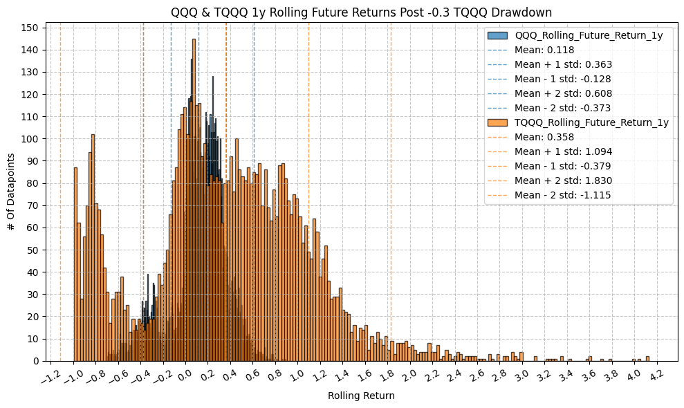

                                  OLS Regression Results
=========================================================================================
Dep. Variable:     TQQQ_Rolling_Future_Return_1y   R-squared:                       0.902
Model:                                       OLS   Adj. R-squared:                  0.902
Method:                            Least Squares   F-statistic:                 5.755e+04
Date:                           Mon, 23 Mar 2026   Prob (F-statistic):               0.00
Time:                                   22:00:13   Log-Likelihood:                 292.28
No. Observations:                           6285   AIC:                            -580.6
Df Residuals:                               6283   BIC:                            -567.1
Df Model:                                      1
Covariance Type:                       nonrobust
================================================================================================
                                   coef    std err          t      P>|t|      [0.025      0.975]
------------------------------------------------------------------------------------------------
const                            0.0222      0.003      6.880      0.000       0.016       0.029
QQQ_Rolling_Future_Return_1y     2.8512      0.012    239.888      0.000       2.828       2.875
==============================================================================
Omnibus:                     1989.506   Durbin-Watson:                   0.043
Prob(Omnibus):                  0.000   Jarque-Bera (JB):             8599.570
Skew:                           1.494   Prob(JB):                         0.00
Kurtosis:                       7.890   Cond. No.                         4.14
==============================================================================

Notes:
[1] Standard Errors assume that the covariance matrix of the errors is correctly specified.
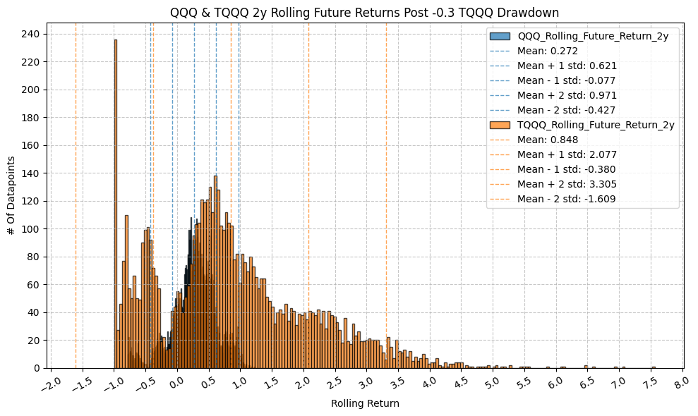

                                  OLS Regression Results
=========================================================================================
Dep. Variable:     TQQQ_Rolling_Future_Return_2y   R-squared:                       0.847
Model:                                       OLS   Adj. R-squared:                  0.847
Method:                            Least Squares   F-statistic:                 3.330e+04
Date:                           Mon, 23 Mar 2026   Prob (F-statistic):               0.00
Time:                                   22:00:15   Log-Likelihood:                -4146.1
No. Observations:                           6033   AIC:                             8296.
Df Residuals:                               6031   BIC:                             8310.
Df Model:                                      1
Covariance Type:                       nonrobust
================================================================================================
                                   coef    std err          t      P>|t|      [0.025      0.975]
------------------------------------------------------------------------------------------------
const                           -0.0321      0.008     -4.090      0.000      -0.048      -0.017
QQQ_Rolling_Future_Return_2y     3.2363      0.018    182.474      0.000       3.202       3.271
==============================================================================
Omnibus:                     1703.989   Durbin-Watson:                   0.019
Prob(Omnibus):                  0.000   Jarque-Bera (JB):             4959.915
Skew:                           1.473   Prob(JB):                         0.00
Kurtosis:                       6.325   Cond. No.                         3.10
==============================================================================

Notes:
[1] Standard Errors assume that the covariance matrix of the errors is correctly specified.


                                  OLS Regression Results
=========================================================================================
Dep. Variable:     TQQQ_Rolling_Future_Return_3y   R-squared:                       0.817
Model:                                       OLS   Adj. R-squared:                  0.816
Method:                            Least Squares   F-statistic:                 2.571e+04
Date:                           Mon, 23 Mar 2026   Prob (F-statistic):               0.00
Time:                                   22:00:16   Log-Likelihood:                -6097.7
No. Observations:                           5781   AIC:                         1.220e+04
Df Residuals:                               5779   BIC:                         1.221e+04
Df Model:                                      1
Covariance Type:                       nonrobust
================================================================================================
                                   coef    std err          t      P>|t|      [0.025      0.975]
------------------------------------------------------------------------------------------------
const                           -0.2501      0.014    -18.444      0.000      -0.277      -0.224
QQQ_Rolling_Future_Return_3y     3.6560      0.023    160.357      0.000       3.611       3.701
==============================================================================
Omnibus:                      879.259   Durbin-Watson:                   0.015
Prob(Omnibus):                  0.000   Jarque-Bera (JB):             1604.922
Skew:                           0.969   Prob(JB):                         0.00
Kurtosis:                       4.706   Cond. No.                         3.05
==============================================================================

Notes:
[1] Standard Errors assume that the covariance matrix of the errors is correctly specified.
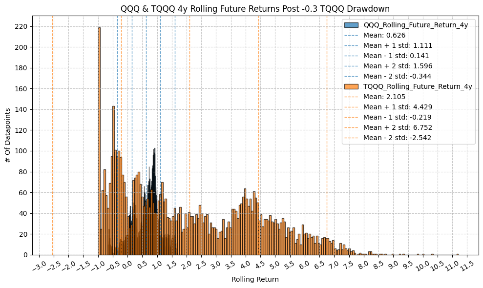

                                  OLS Regression Results
=========================================================================================
Dep. Variable:     TQQQ_Rolling_Future_Return_4y   R-squared:                       0.785
Model:                                       OLS   Adj. R-squared:                  0.785
Method:                            Least Squares   F-statistic:                 2.013e+04
Date:                           Mon, 23 Mar 2026   Prob (F-statistic):               0.00
Time:                                   22:00:18   Log-Likelihood:                -8262.7
No. Observations:                           5529   AIC:                         1.653e+04
Df Residuals:                               5527   BIC:                         1.654e+04
Df Model:                                      1
Covariance Type:                       nonrobust
================================================================================================
                                   coef    std err          t      P>|t|      [0.025      0.975]
------------------------------------------------------------------------------------------------
const                           -0.5505      0.024    -23.246      0.000      -0.597      -0.504
QQQ_Rolling_Future_Return_4y     4.2437      0.030    141.872      0.000       4.185       4.302
==============================================================================
Omnibus:                       73.818   Durbin-Watson:                   0.010
Prob(Omnibus):                  0.000   Jarque-Bera (JB):               55.847
Skew:                           0.155   Prob(JB):                     7.46e-13
Kurtosis:                       2.617   Cond. No.                         3.02
==============================================================================

Notes:
[1] Standard Errors assume that the covariance matrix of the errors is correctly specified.

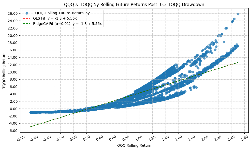
                                  OLS Regression Results
=========================================================================================
Dep. Variable:     TQQQ_Rolling_Future_Return_5y   R-squared:                       0.747
Model:                                       OLS   Adj. R-squared:                  0.747
Method:                            Least Squares   F-statistic:                 1.560e+04
Date:                           Mon, 23 Mar 2026   Prob (F-statistic):               0.00
Time:                                   22:00:20   Log-Likelihood:                -11446.
No. Observations:                           5277   AIC:                         2.290e+04
Df Residuals:                               5275   BIC:                         2.291e+04
Df Model:                                      1
Covariance Type:                       nonrobust
================================================================================================
                                   coef    std err          t      P>|t|      [0.025      0.975]
------------------------------------------------------------------------------------------------
const                           -1.3180      0.049    -26.870      0.000      -1.414      -1.222
QQQ_Rolling_Future_Return_5y     5.5645      0.045    124.886      0.000       5.477       5.652
==============================================================================
Omnibus:                      246.937   Durbin-Watson:                   0.009
Prob(Omnibus):                  0.000   Jarque-Bera (JB):              368.613
Skew:                           0.425   Prob(JB):                     9.05e-81
Kurtosis:                       3.977   Cond. No.                         3.05
==============================================================================

Notes:
[1] Standard Errors assume that the covariance matrix of the errors is correctly specified.


                                  OLS Regression Results
=========================================================================================
Dep. Variable:     TQQQ_Rolling_Future_Return_1d   R-squared:                       0.999
Model:                                       OLS   Adj. R-squared:                  0.999
Method:                            Least Squares   F-statistic:                 6.390e+06
Date:                           Mon, 23 Mar 2026   Prob (F-statistic):               0.00
Time:                                   22:00:22   Log-Likelihood:                 32859.
No. Observations:                           6525   AIC:                        -6.571e+04
Df Residuals:                               6523   BIC:                        -6.570e+04
Df Model:                                      1
Covariance Type:                       nonrobust
================================================================================================
                                   coef    std err          t      P>|t|      [0.025      0.975]
------------------------------------------------------------------------------------------------
const                        -5.353e-05   1.95e-05     -2.748      0.006   -9.17e-05   -1.53e-05
QQQ_Rolling_Future_Return_1d     2.9552      0.001   2527.781      0.000       2.953       2.957
==============================================================================
Omnibus:                     9680.797   Durbin-Watson:                   2.565
Prob(Omnibus):                  0.000   Jarque-Bera (JB):         38804068.521
Skew:                          -8.106   Prob(JB):                         0.00
Kurtosis:                     380.445   Cond. No.                         60.0
==============================================================================

Notes:
[1] Standard Errors assume that the covariance matrix of the errors is correctly specified.
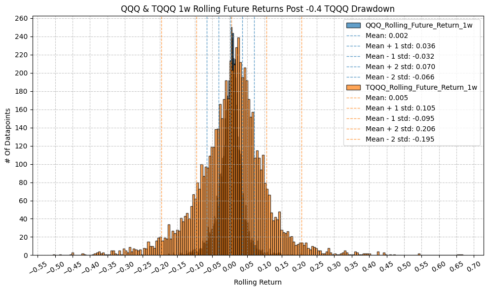
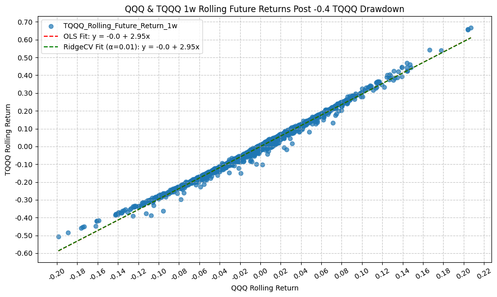
                                  OLS Regression Results
=========================================================================================
Dep. Variable:     TQQQ_Rolling_Future_Return_1w   R-squared:                       0.994
Model:                                       OLS   Adj. R-squared:                  0.994
Method:                            Least Squares   F-statistic:                 1.119e+06
Date:                           Mon, 23 Mar 2026   Prob (F-statistic):               0.00
Time:                                   22:00:24   Log-Likelihood:                 22546.
No. Observations:                           6521   AIC:                        -4.509e+04
Df Residuals:                               6519   BIC:                        -4.508e+04
Df Model:                                      1
Covariance Type:                       nonrobust
================================================================================================
                                   coef    std err          t      P>|t|      [0.025      0.975]
------------------------------------------------------------------------------------------------
const                           -0.0008   9.46e-05     -8.597      0.000      -0.001      -0.001
QQQ_Rolling_Future_Return_1w     2.9536      0.003   1057.873      0.000       2.948       2.959
==============================================================================
Omnibus:                     3596.565   Durbin-Watson:                   0.881
Prob(Omnibus):                  0.000   Jarque-Bera (JB):           404696.936
Skew:                          -1.687   Prob(JB):                         0.00
Kurtosis:                      41.446   Cond. No.                         29.6
==============================================================================

Notes:
[1] Standard Errors assume that the covariance matrix of the errors is correctly specified.


                                  OLS Regression Results
=========================================================================================
Dep. Variable:     TQQQ_Rolling_Future_Return_1m   R-squared:                       0.983
Model:                                       OLS   Adj. R-squared:                  0.983
Method:                            Least Squares   F-statistic:                 3.664e+05
Date:                           Mon, 23 Mar 2026   Prob (F-statistic):               0.00
Time:                                   22:00:26   Log-Likelihood:                 14632.
No. Observations:                           6505   AIC:                        -2.926e+04
Df Residuals:                               6503   BIC:                        -2.925e+04
Df Model:                                      1
Covariance Type:                       nonrobust
================================================================================================
                                   coef    std err          t      P>|t|      [0.025      0.975]
------------------------------------------------------------------------------------------------
const                           -0.0035      0.000    -11.058      0.000      -0.004      -0.003
QQQ_Rolling_Future_Return_1m     2.9151      0.005    605.320      0.000       2.906       2.925
==============================================================================
Omnibus:                     1512.367   Durbin-Watson:                   0.297
Prob(Omnibus):                  0.000   Jarque-Bera (JB):            83017.003
Skew:                           0.063   Prob(JB):                         0.00
Kurtosis:                      20.501   Cond. No.                         15.2
==============================================================================

Notes:
[1] Standard Errors assume that the covariance matrix of the errors is correctly specified.
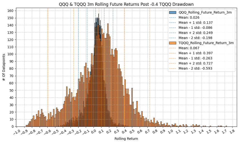

                                  OLS Regression Results
=========================================================================================
Dep. Variable:     TQQQ_Rolling_Future_Return_3m   R-squared:                       0.961
Model:                                       OLS   Adj. R-squared:                  0.961
Method:                            Least Squares   F-statistic:                 1.592e+05
Date:                           Mon, 23 Mar 2026   Prob (F-statistic):               0.00
Time:                                   22:00:28   Log-Likelihood:                 8479.8
No. Observations:                           6463   AIC:                        -1.696e+04
Df Residuals:                               6461   BIC:                        -1.694e+04
Df Model:                                      1
Covariance Type:                       nonrobust
================================================================================================
                                   coef    std err          t      P>|t|      [0.025      0.975]
------------------------------------------------------------------------------------------------
const                           -0.0066      0.001     -7.911      0.000      -0.008      -0.005
QQQ_Rolling_Future_Return_3m     2.8926      0.007    399.038      0.000       2.878       2.907
==============================================================================
Omnibus:                     1379.365   Durbin-Watson:                   0.101
Prob(Omnibus):                  0.000   Jarque-Bera (JB):            15633.345
Skew:                           0.693   Prob(JB):                         0.00
Kurtosis:                      10.492   Cond. No.                         8.95
==============================================================================

Notes:
[1] Standard Errors assume that the covariance matrix of the errors is correctly specified.

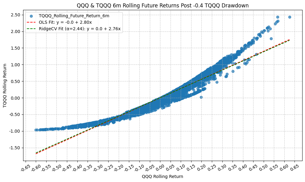
                                  OLS Regression Results
=========================================================================================
Dep. Variable:     TQQQ_Rolling_Future_Return_6m   R-squared:                       0.931
Model:                                       OLS   Adj. R-squared:                  0.931
Method:                            Least Squares   F-statistic:                 8.660e+04
Date:                           Mon, 23 Mar 2026   Prob (F-statistic):               0.00
Time:                                   22:00:29   Log-Likelihood:                 4309.6
No. Observations:                           6400   AIC:                            -8615.
Df Residuals:                               6398   BIC:                            -8602.
Df Model:                                      1
Covariance Type:                       nonrobust
================================================================================================
                                   coef    std err          t      P>|t|      [0.025      0.975]
------------------------------------------------------------------------------------------------
const                        -7.935e-05      0.002     -0.049      0.961      -0.003       0.003
QQQ_Rolling_Future_Return_6m     2.8038      0.010    294.287      0.000       2.785       2.822
==============================================================================
Omnibus:                     1641.226   Durbin-Watson:                   0.057
Prob(Omnibus):                  0.000   Jarque-Bera (JB):             8159.048
Skew:                           1.148   Prob(JB):                         0.00
Kurtosis:                       8.033   Cond. No.                         6.19
==============================================================================

Notes:
[1] Standard Errors assume that the covariance matrix of the errors is correctly specified.


                                  OLS Regression Results
=========================================================================================
Dep. Variable:     TQQQ_Rolling_Future_Return_1y   R-squared:                       0.902
Model:                                       OLS   Adj. R-squared:                  0.902
Method:                            Least Squares   F-statistic:                 5.795e+04
Date:                           Mon, 23 Mar 2026   Prob (F-statistic):               0.00
Time:                                   22:00:31   Log-Likelihood:                 326.52
No. Observations:                           6274   AIC:                            -649.0
Df Residuals:                               6272   BIC:                            -635.5
Df Model:                                      1
Covariance Type:                       nonrobust
================================================================================================
                                   coef    std err          t      P>|t|      [0.025      0.975]
------------------------------------------------------------------------------------------------
const                            0.0209      0.003      6.496      0.000       0.015       0.027
QQQ_Rolling_Future_Return_1y     2.8615      0.012    240.734      0.000       2.838       2.885
==============================================================================
Omnibus:                     1986.979   Durbin-Watson:                   0.039
Prob(Omnibus):                  0.000   Jarque-Bera (JB):             8588.911
Skew:                           1.495   Prob(JB):                         0.00
Kurtosis:                       7.890   Cond. No.                         4.16
==============================================================================

Notes:
[1] Standard Errors assume that the covariance matrix of the errors is correctly specified.

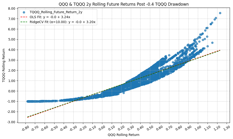
                                  OLS Regression Results
=========================================================================================
Dep. Variable:     TQQQ_Rolling_Future_Return_2y   R-squared:                       0.847
Model:                                       OLS   Adj. R-squared:                  0.847
Method:                            Least Squares   F-statistic:                 3.332e+04
Date:                           Mon, 23 Mar 2026   Prob (F-statistic):               0.00
Time:                                   22:00:33   Log-Likelihood:                -4126.3
No. Observations:                           6022   AIC:                             8257.
Df Residuals:                               6020   BIC:                             8270.
Df Model:                                      1
Covariance Type:                       nonrobust
================================================================================================
                                   coef    std err          t      P>|t|      [0.025      0.975]
------------------------------------------------------------------------------------------------
const                           -0.0349      0.008     -4.437      0.000      -0.050      -0.019
QQQ_Rolling_Future_Return_2y     3.2436      0.018    182.525      0.000       3.209       3.278
==============================================================================
Omnibus:                     1713.005   Durbin-Watson:                   0.018
Prob(Omnibus):                  0.000   Jarque-Bera (JB):             5037.679
Skew:                           1.479   Prob(JB):                         0.00
Kurtosis:                       6.365   Cond. No.                         3.11
==============================================================================

Notes:
[1] Standard Errors assume that the covariance matrix of the errors is correctly specified.
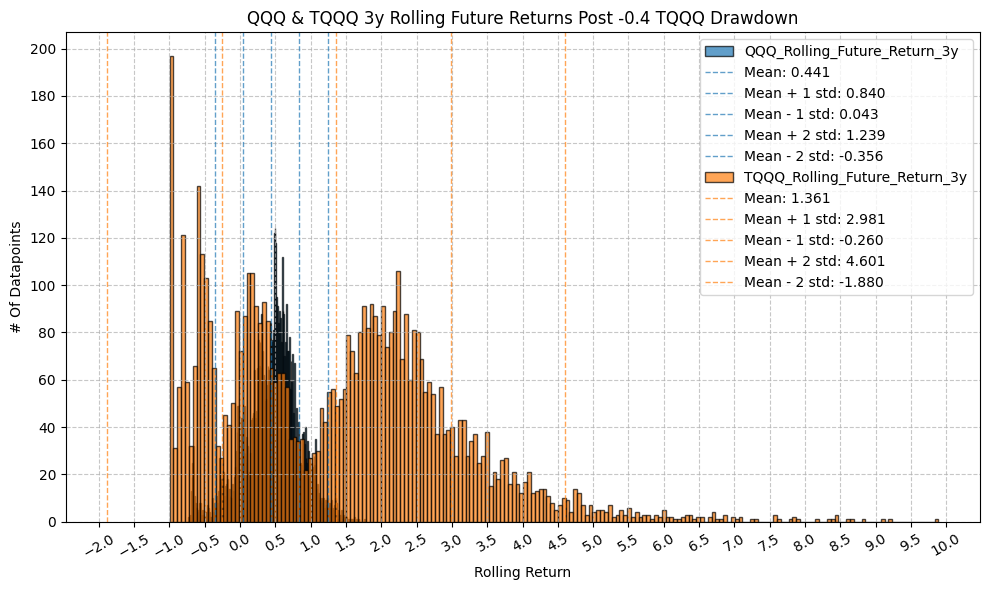

                                  OLS Regression Results
=========================================================================================
Dep. Variable:     TQQQ_Rolling_Future_Return_3y   R-squared:                       0.818
Model:                                       OLS   Adj. R-squared:                  0.818
Method:                            Least Squares   F-statistic:                 2.586e+04
Date:                           Mon, 23 Mar 2026   Prob (F-statistic):               0.00
Time:                                   22:00:34   Log-Likelihood:                -6062.3
No. Observations:                           5770   AIC:                         1.213e+04
Df Residuals:                               5768   BIC:                         1.214e+04
Df Model:                                      1
Covariance Type:                       nonrobust
================================================================================================
                                   coef    std err          t      P>|t|      [0.025      0.975]
------------------------------------------------------------------------------------------------
const                           -0.2617      0.014    -19.250      0.000      -0.288      -0.235
QQQ_Rolling_Future_Return_3y     3.6758      0.023    160.808      0.000       3.631       3.721
==============================================================================
Omnibus:                      872.524   Durbin-Watson:                   0.015
Prob(Omnibus):                  0.000   Jarque-Bera (JB):             1594.376
Skew:                           0.963   Prob(JB):                         0.00
Kurtosis:                       4.709   Cond. No.                         3.07
==============================================================================

Notes:
[1] Standard Errors assume that the covariance matrix of the errors is correctly specified.
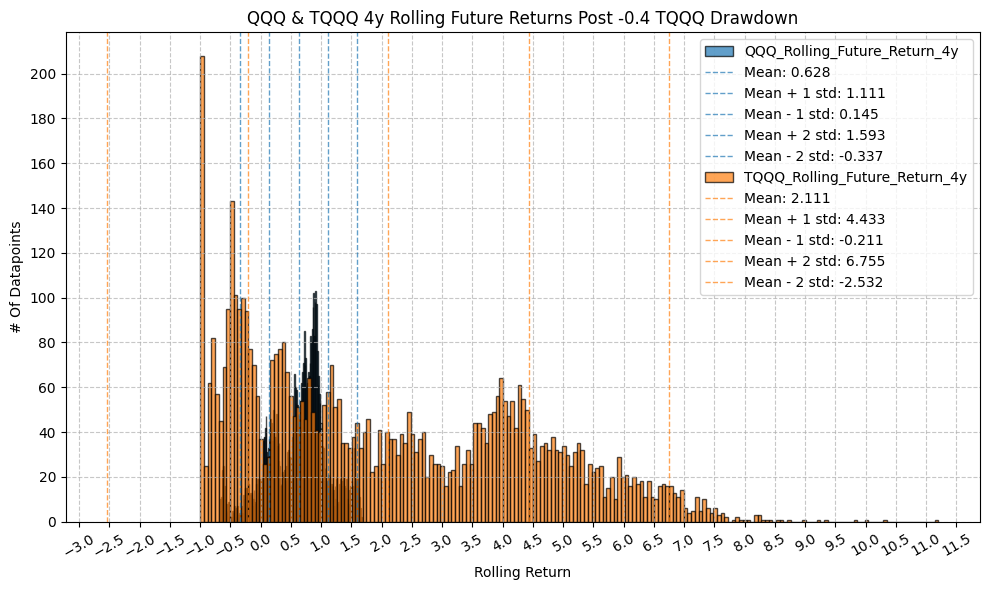

                                  OLS Regression Results
=========================================================================================
Dep. Variable:     TQQQ_Rolling_Future_Return_4y   R-squared:                       0.785
Model:                                       OLS   Adj. R-squared:                  0.785
Method:                            Least Squares   F-statistic:                 2.015e+04
Date:                           Mon, 23 Mar 2026   Prob (F-statistic):               0.00
Time:                                   22:00:37   Log-Likelihood:                -8235.5
No. Observations:                           5518   AIC:                         1.647e+04
Df Residuals:                               5516   BIC:                         1.649e+04
Df Model:                                      1
Covariance Type:                       nonrobust
================================================================================================
                                   coef    std err          t      P>|t|      [0.025      0.975]
------------------------------------------------------------------------------------------------
const                           -0.5654      0.024    -23.773      0.000      -0.612      -0.519
QQQ_Rolling_Future_Return_4y     4.2617      0.030    141.942      0.000       4.203       4.321
==============================================================================
Omnibus:                       68.572   Durbin-Watson:                   0.010
Prob(Omnibus):                  0.000   Jarque-Bera (JB):               52.789
Skew:                           0.153   Prob(JB):                     3.44e-12
Kurtosis:                       2.631   Cond. No.                         3.04
==============================================================================

Notes:
[1] Standard Errors assume that the covariance matrix of the errors is correctly specified.
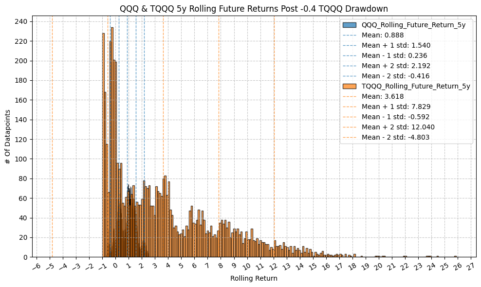

                                  OLS Regression Results
=========================================================================================
Dep. Variable:     TQQQ_Rolling_Future_Return_5y   R-squared:                       0.748
Model:                                       OLS   Adj. R-squared:                  0.748
Method:                            Least Squares   F-statistic:                 1.561e+04
Date:                           Mon, 23 Mar 2026   Prob (F-statistic):               0.00
Time:                                   22:00:38   Log-Likelihood:                -11415.
No. Observations:                           5266   AIC:                         2.283e+04
Df Residuals:                               5264   BIC:                         2.285e+04
Df Model:                                      1
Covariance Type:                       nonrobust
================================================================================================
                                   coef    std err          t      P>|t|      [0.025      0.975]
------------------------------------------------------------------------------------------------
const                           -1.3430      0.049    -27.264      0.000      -1.440      -1.246
QQQ_Rolling_Future_Return_5y     5.5855      0.045    124.935      0.000       5.498       5.673
==============================================================================
Omnibus:                      242.424   Durbin-Watson:                   0.009
Prob(Omnibus):                  0.000   Jarque-Bera (JB):              363.603
Skew:                           0.418   Prob(JB):                     1.11e-79
Kurtosis:                       3.979   Cond. No.                         3.07
==============================================================================

Notes:
[1] Standard Errors assume that the covariance matrix of the errors is correctly specified.


                                  OLS Regression Results
=========================================================================================
Dep. Variable:     TQQQ_Rolling_Future_Return_1d   R-squared:                       0.999
Model:                                       OLS   Adj. R-squared:                  0.999
Method:                            Least Squares   F-statistic:                 6.259e+06
Date:                           Mon, 23 Mar 2026   Prob (F-statistic):               0.00
Time:                                   22:00:40   Log-Likelihood:                 32521.
No. Observations:                           6462   AIC:                        -6.504e+04
Df Residuals:                               6460   BIC:                        -6.502e+04
Df Model:                                      1
Covariance Type:                       nonrobust
================================================================================================
                                   coef    std err          t      P>|t|      [0.025      0.975]
------------------------------------------------------------------------------------------------
const                        -4.963e-05   1.96e-05     -2.527      0.012   -8.81e-05   -1.11e-05
QQQ_Rolling_Future_Return_1d     2.9550      0.001   2501.868      0.000       2.953       2.957
==============================================================================
Omnibus:                     9587.532   Durbin-Watson:                   2.567
Prob(Omnibus):                  0.000   Jarque-Bera (JB):         38153267.854
Skew:                          -8.108   Prob(JB):                         0.00
Kurtosis:                     379.084   Cond. No.                         60.2
==============================================================================

Notes:
[1] Standard Errors assume that the covariance matrix of the errors is correctly specified.
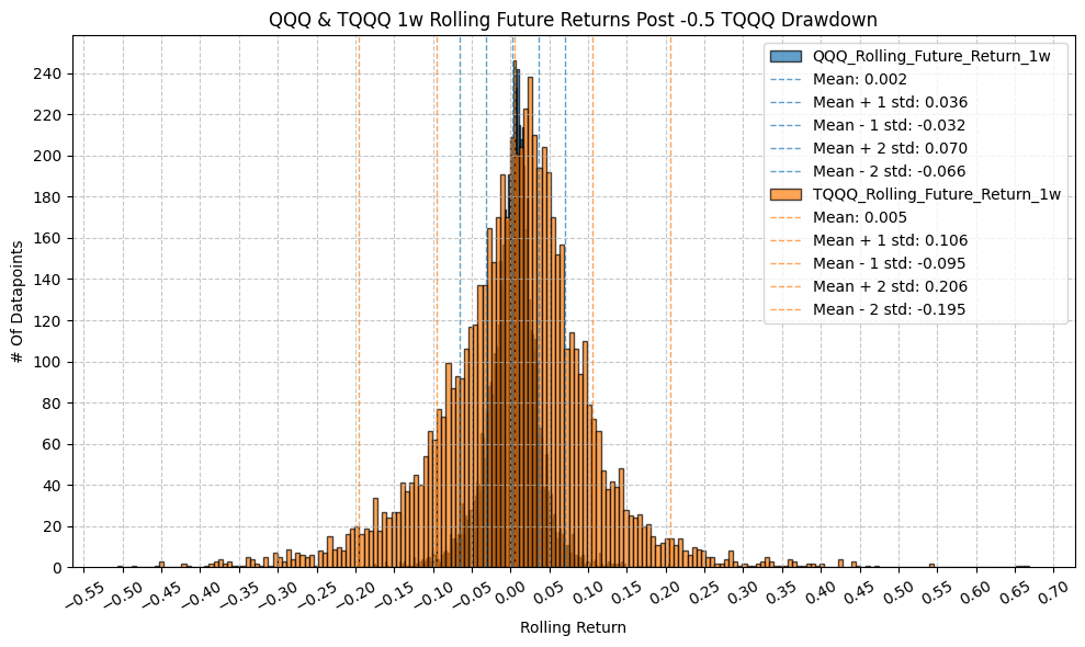

                                  OLS Regression Results
=========================================================================================
Dep. Variable:     TQQQ_Rolling_Future_Return_1w   R-squared:                       0.994
Model:                                       OLS   Adj. R-squared:                  0.994
Method:                            Least Squares   F-statistic:                 1.110e+06
Date:                           Mon, 23 Mar 2026   Prob (F-statistic):               0.00
Time:                                   22:00:42   Log-Likelihood:                 22331.
No. Observations:                           6458   AIC:                        -4.466e+04
Df Residuals:                               6456   BIC:                        -4.464e+04
Df Model:                                      1
Covariance Type:                       nonrobust
================================================================================================
                                   coef    std err          t      P>|t|      [0.025      0.975]
------------------------------------------------------------------------------------------------
const                           -0.0008    9.5e-05     -8.200      0.000      -0.001      -0.001
QQQ_Rolling_Future_Return_1w     2.9530      0.003   1053.776      0.000       2.947       2.958
==============================================================================
Omnibus:                     3543.021   Durbin-Watson:                   0.887
Prob(Omnibus):                  0.000   Jarque-Bera (JB):           403213.894
Skew:                          -1.668   Prob(JB):                         0.00
Kurtosis:                      41.566   Cond. No.                         29.5
==============================================================================

Notes:
[1] Standard Errors assume that the covariance matrix of the errors is correctly specified.


                                  OLS Regression Results
=========================================================================================
Dep. Variable:     TQQQ_Rolling_Future_Return_1m   R-squared:                       0.983
Model:                                       OLS   Adj. R-squared:                  0.983
Method:                            Least Squares   F-statistic:                 3.617e+05
Date:                           Mon, 23 Mar 2026   Prob (F-statistic):               0.00
Time:                                   22:00:44   Log-Likelihood:                 14468.
No. Observations:                           6442   AIC:                        -2.893e+04
Df Residuals:                               6440   BIC:                        -2.892e+04
Df Model:                                      1
Covariance Type:                       nonrobust
================================================================================================
                                   coef    std err          t      P>|t|      [0.025      0.975]
------------------------------------------------------------------------------------------------
const                           -0.0034      0.000    -10.631      0.000      -0.004      -0.003
QQQ_Rolling_Future_Return_1m     2.9145      0.005    601.447      0.000       2.905       2.924
==============================================================================
Omnibus:                     1492.448   Durbin-Watson:                   0.295
Prob(Omnibus):                  0.000   Jarque-Bera (JB):            81230.387
Skew:                           0.050   Prob(JB):                         0.00
Kurtosis:                      20.396   Cond. No.                         15.2
==============================================================================

Notes:
[1] Standard Errors assume that the covariance matrix of the errors is correctly specified.


                                  OLS Regression Results
=========================================================================================
Dep. Variable:     TQQQ_Rolling_Future_Return_3m   R-squared:                       0.961
Model:                                       OLS   Adj. R-squared:                  0.961
Method:                            Least Squares   F-statistic:                 1.589e+05
Date:                           Mon, 23 Mar 2026   Prob (F-statistic):               0.00
Time:                                   22:00:46   Log-Likelihood:                 8433.0
No. Observations:                           6427   AIC:                        -1.686e+04
Df Residuals:                               6425   BIC:                        -1.685e+04
Df Model:                                      1
Covariance Type:                       nonrobust
================================================================================================
                                   coef    std err          t      P>|t|      [0.025      0.975]
------------------------------------------------------------------------------------------------
const                           -0.0063      0.001     -7.555      0.000      -0.008      -0.005
QQQ_Rolling_Future_Return_3m     2.8921      0.007    398.661      0.000       2.878       2.906
==============================================================================
Omnibus:                     1377.477   Durbin-Watson:                   0.101
Prob(Omnibus):                  0.000   Jarque-Bera (JB):            15521.588
Skew:                           0.699   Prob(JB):                         0.00
Kurtosis:                      10.484   Cond. No.                         8.93
==============================================================================

Notes:
[1] Standard Errors assume that the covariance matrix of the errors is correctly specified.
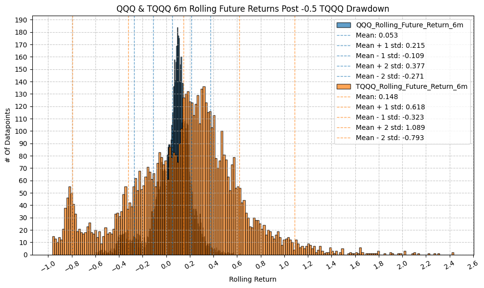

                                  OLS Regression Results
=========================================================================================
Dep. Variable:     TQQQ_Rolling_Future_Return_6m   R-squared:                       0.931
Model:                                       OLS   Adj. R-squared:                  0.931
Method:                            Least Squares   F-statistic:                 8.678e+04
Date:                           Mon, 23 Mar 2026   Prob (F-statistic):               0.00
Time:                                   22:00:48   Log-Likelihood:                 4316.3
No. Observations:                           6397   AIC:                            -8629.
Df Residuals:                               6395   BIC:                            -8615.
Df Model:                                      1
Covariance Type:                       nonrobust
================================================================================================
                                   coef    std err          t      P>|t|      [0.025      0.975]
------------------------------------------------------------------------------------------------
const                         3.496e-05      0.002      0.022      0.983      -0.003       0.003
QQQ_Rolling_Future_Return_6m     2.8039      0.010    294.583      0.000       2.785       2.823
==============================================================================
Omnibus:                     1657.019   Durbin-Watson:                   0.055
Prob(Omnibus):                  0.000   Jarque-Bera (JB):             8164.864
Skew:                           1.163   Prob(JB):                         0.00
Kurtosis:                       8.022   Cond. No.                         6.19
==============================================================================

Notes:
[1] Standard Errors assume that the covariance matrix of the errors is correctly specified.
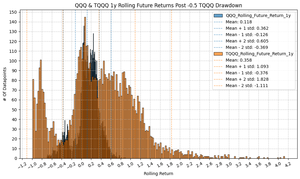

                                  OLS Regression Results
=========================================================================================
Dep. Variable:     TQQQ_Rolling_Future_Return_1y   R-squared:                       0.902
Model:                                       OLS   Adj. R-squared:                  0.902
Method:                            Least Squares   F-statistic:                 5.802e+04
Date:                           Mon, 23 Mar 2026   Prob (F-statistic):               0.00
Time:                                   22:00:49   Log-Likelihood:                 334.10
No. Observations:                           6271   AIC:                            -664.2
Df Residuals:                               6269   BIC:                            -650.7
Df Model:                                      1
Covariance Type:                       nonrobust
================================================================================================
                                   coef    std err          t      P>|t|      [0.025      0.975]
------------------------------------------------------------------------------------------------
const                            0.0204      0.003      6.337      0.000       0.014       0.027
QQQ_Rolling_Future_Return_1y     2.8641      0.012    240.870      0.000       2.841       2.887
==============================================================================
Omnibus:                     1985.718   Durbin-Watson:                   0.038
Prob(Omnibus):                  0.000   Jarque-Bera (JB):             8605.916
Skew:                           1.494   Prob(JB):                         0.00
Kurtosis:                       7.900   Cond. No.                         4.16
==============================================================================

Notes:
[1] Standard Errors assume that the covariance matrix of the errors is correctly specified.


                                  OLS Regression Results
=========================================================================================
Dep. Variable:     TQQQ_Rolling_Future_Return_2y   R-squared:                       0.847
Model:                                       OLS   Adj. R-squared:                  0.847
Method:                            Least Squares   F-statistic:                 3.334e+04
Date:                           Mon, 23 Mar 2026   Prob (F-statistic):               0.00
Time:                                   22:00:51   Log-Likelihood:                -4119.1
No. Observations:                           6019   AIC:                             8242.
Df Residuals:                               6017   BIC:                             8256.
Df Model:                                      1
Covariance Type:                       nonrobust
================================================================================================
                                   coef    std err          t      P>|t|      [0.025      0.975]
------------------------------------------------------------------------------------------------
const                           -0.0364      0.008     -4.622      0.000      -0.052      -0.021
QQQ_Rolling_Future_Return_2y     3.2472      0.018    182.598      0.000       3.212       3.282
==============================================================================
Omnibus:                     1718.217   Durbin-Watson:                   0.018
Prob(Omnibus):                  0.000   Jarque-Bera (JB):             5077.476
Skew:                           1.483   Prob(JB):                         0.00
Kurtosis:                       6.384   Cond. No.                         3.12
==============================================================================

Notes:
[1] Standard Errors assume that the covariance matrix of the errors is correctly specified.

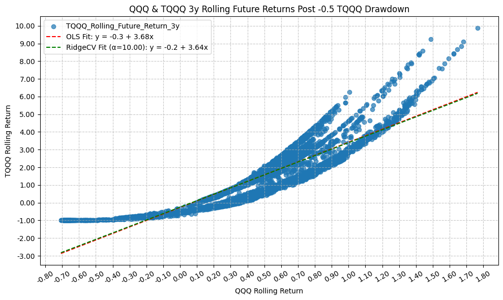
                                  OLS Regression Results
=========================================================================================
Dep. Variable:     TQQQ_Rolling_Future_Return_3y   R-squared:                       0.818
Model:                                       OLS   Adj. R-squared:                  0.818
Method:                            Least Squares   F-statistic:                 2.593e+04
Date:                           Mon, 23 Mar 2026   Prob (F-statistic):               0.00
Time:                                   22:00:53   Log-Likelihood:                -6049.6
No. Observations:                           5767   AIC:                         1.210e+04
Df Residuals:                               5765   BIC:                         1.212e+04
Df Model:                                      1
Covariance Type:                       nonrobust
================================================================================================
                                   coef    std err          t      P>|t|      [0.025      0.975]
------------------------------------------------------------------------------------------------
const                           -0.2658      0.014    -19.545      0.000      -0.292      -0.239
QQQ_Rolling_Future_Return_3y     3.6829      0.023    161.036      0.000       3.638       3.728
==============================================================================
Omnibus:                      869.247   Durbin-Watson:                   0.015
Prob(Omnibus):                  0.000   Jarque-Bera (JB):             1588.727
Skew:                           0.960   Prob(JB):                         0.00
Kurtosis:                       4.709   Cond. No.                         3.08
==============================================================================

Notes:
[1] Standard Errors assume that the covariance matrix of the errors is correctly specified.
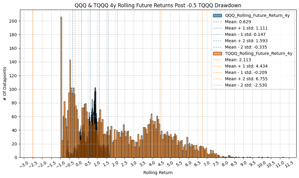
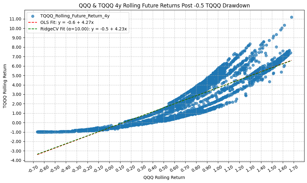
                                  OLS Regression Results
=========================================================================================
Dep. Variable:     TQQQ_Rolling_Future_Return_4y   R-squared:                       0.785
Model:                                       OLS   Adj. R-squared:                  0.785
Method:                            Least Squares   F-statistic:                 2.017e+04
Date:                           Mon, 23 Mar 2026   Prob (F-statistic):               0.00
Time:                                   22:00:55   Log-Likelihood:                -8226.6
No. Observations:                           5515   AIC:                         1.646e+04
Df Residuals:                               5513   BIC:                         1.647e+04
Df Model:                                      1
Covariance Type:                       nonrobust
================================================================================================
                                   coef    std err          t      P>|t|      [0.025      0.975]
------------------------------------------------------------------------------------------------
const                           -0.5704      0.024    -23.957      0.000      -0.617      -0.524
QQQ_Rolling_Future_Return_4y     4.2678      0.030    142.009      0.000       4.209       4.327
==============================================================================
Omnibus:                       66.838   Durbin-Watson:                   0.010
Prob(Omnibus):                  0.000   Jarque-Bera (JB):               51.664
Skew:                           0.151   Prob(JB):                     6.04e-12
Kurtosis:                       2.635   Cond. No.                         3.05
==============================================================================

Notes:
[1] Standard Errors assume that the covariance matrix of the errors is correctly specified.
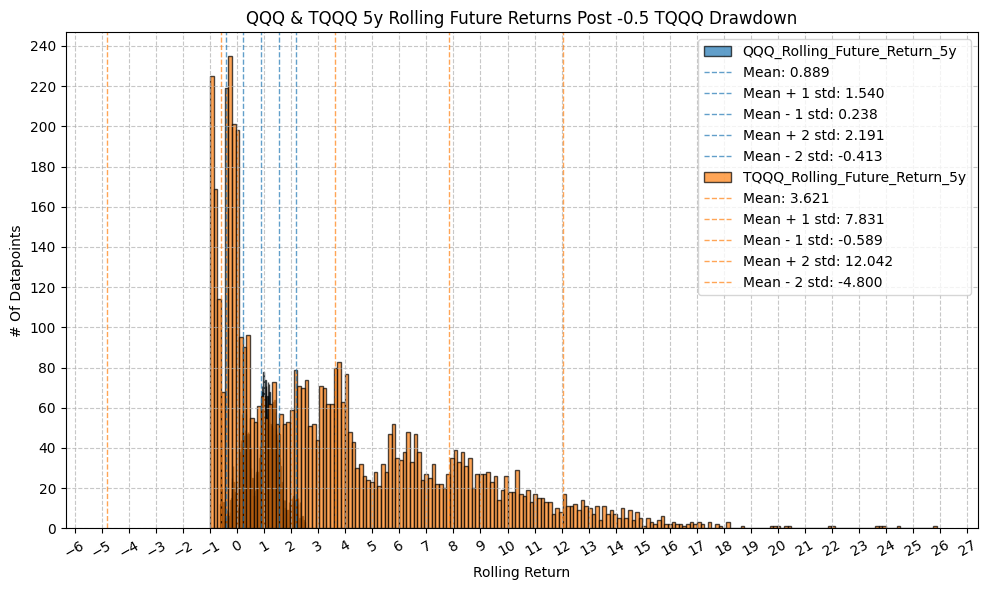

                                  OLS Regression Results
=========================================================================================
Dep. Variable:     TQQQ_Rolling_Future_Return_5y   R-squared:                       0.748
Model:                                       OLS   Adj. R-squared:                  0.748
Method:                            Least Squares   F-statistic:                 1.562e+04
Date:                           Mon, 23 Mar 2026   Prob (F-statistic):               0.00
Time:                                   22:00:57   Log-Likelihood:                -11405.
No. Observations:                           5263   AIC:                         2.281e+04
Df Residuals:                               5261   BIC:                         2.283e+04
Df Model:                                      1
Covariance Type:                       nonrobust
================================================================================================
                                   coef    std err          t      P>|t|      [0.025      0.975]
------------------------------------------------------------------------------------------------
const                           -1.3518      0.049    -27.413      0.000      -1.448      -1.255
QQQ_Rolling_Future_Return_5y     5.5930      0.045    124.992      0.000       5.505       5.681
==============================================================================
Omnibus:                      240.577   Durbin-Watson:                   0.009
Prob(Omnibus):                  0.000   Jarque-Bera (JB):              361.692
Skew:                           0.415   Prob(JB):                     2.88e-79
Kurtosis:                       3.980   Cond. No.                         3.08
==============================================================================

Notes:
[1] Standard Errors assume that the covariance matrix of the errors is correctly specified.


                                  OLS Regression Results
=========================================================================================
Dep. Variable:     TQQQ_Rolling_Future_Return_1d   R-squared:                       0.999
Model:                                       OLS   Adj. R-squared:                  0.999
Method:                            Least Squares   F-statistic:                 6.000e+06
Date:                           Mon, 23 Mar 2026   Prob (F-statistic):               0.00
Time:                                   22:00:59   Log-Likelihood:                 31538.
No. Observations:                           6281   AIC:                        -6.307e+04
Df Residuals:                               6279   BIC:                        -6.306e+04
Df Model:                                      1
Covariance Type:                       nonrobust
================================================================================================
                                   coef    std err          t      P>|t|      [0.025      0.975]
------------------------------------------------------------------------------------------------
const                        -4.239e-05   2.02e-05     -2.103      0.035   -8.19e-05   -2.88e-06
QQQ_Rolling_Future_Return_1d     2.9548      0.001   2449.504      0.000       2.952       2.957
==============================================================================
Omnibus:                     9289.579   Durbin-Watson:                   2.569
Prob(Omnibus):                  0.000   Jarque-Bera (JB):         35733225.202
Skew:                          -8.060   Prob(JB):                         0.00
Kurtosis:                     372.159   Cond. No.                         59.9
==============================================================================

Notes:
[1] Standard Errors assume that the covariance matrix of the errors is correctly specified.


                                  OLS Regression Results
=========================================================================================
Dep. Variable:     TQQQ_Rolling_Future_Return_1w   R-squared:                       0.994
Model:                                       OLS   Adj. R-squared:                  0.994
Method:                            Least Squares   F-statistic:                 1.076e+06
Date:                           Mon, 23 Mar 2026   Prob (F-statistic):               0.00
Time:                                   22:01:00   Log-Likelihood:                 21679.
No. Observations:                           6281   AIC:                        -4.335e+04
Df Residuals:                               6279   BIC:                        -4.334e+04
Df Model:                                      1
Covariance Type:                       nonrobust
================================================================================================
                                   coef    std err          t      P>|t|      [0.025      0.975]
------------------------------------------------------------------------------------------------
const                           -0.0007    9.7e-05     -7.559      0.000      -0.001      -0.001
QQQ_Rolling_Future_Return_1w     2.9525      0.003   1037.518      0.000       2.947       2.958
==============================================================================
Omnibus:                     3409.174   Durbin-Watson:                   0.895
Prob(Omnibus):                  0.000   Jarque-Bera (JB):           384856.284
Skew:                          -1.639   Prob(JB):                         0.00
Kurtosis:                      41.207   Cond. No.                         29.4
==============================================================================

Notes:
[1] Standard Errors assume that the covariance matrix of the errors is correctly specified.

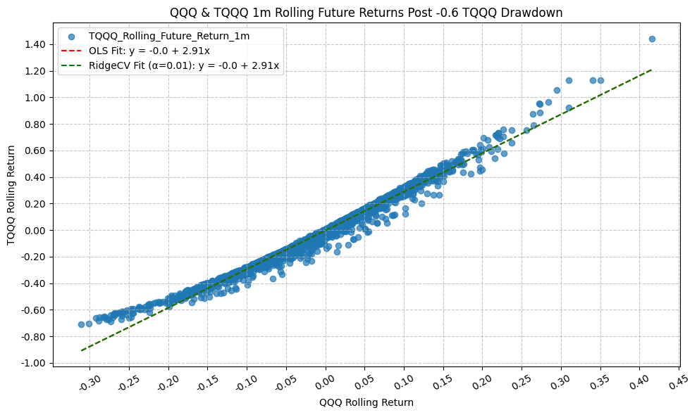
                                  OLS Regression Results
=========================================================================================
Dep. Variable:     TQQQ_Rolling_Future_Return_1m   R-squared:                       0.982
Model:                                       OLS   Adj. R-squared:                  0.982
Method:                            Least Squares   F-statistic:                 3.507e+05
Date:                           Mon, 23 Mar 2026   Prob (F-statistic):               0.00
Time:                                   22:01:02   Log-Likelihood:                 14071.
No. Observations:                           6281   AIC:                        -2.814e+04
Df Residuals:                               6279   BIC:                        -2.812e+04
Df Model:                                      1
Covariance Type:                       nonrobust
================================================================================================
                                   coef    std err          t      P>|t|      [0.025      0.975]
------------------------------------------------------------------------------------------------
const                           -0.0032      0.000     -9.799      0.000      -0.004      -0.003
QQQ_Rolling_Future_Return_1m     2.9141      0.005    592.215      0.000       2.904       2.924
==============================================================================
Omnibus:                     1452.768   Durbin-Watson:                   0.296
Prob(Omnibus):                  0.000   Jarque-Bera (JB):            78418.997
Skew:                           0.053   Prob(JB):                         0.00
Kurtosis:                      20.310   Cond. No.                         15.1
==============================================================================

Notes:
[1] Standard Errors assume that the covariance matrix of the errors is correctly specified.

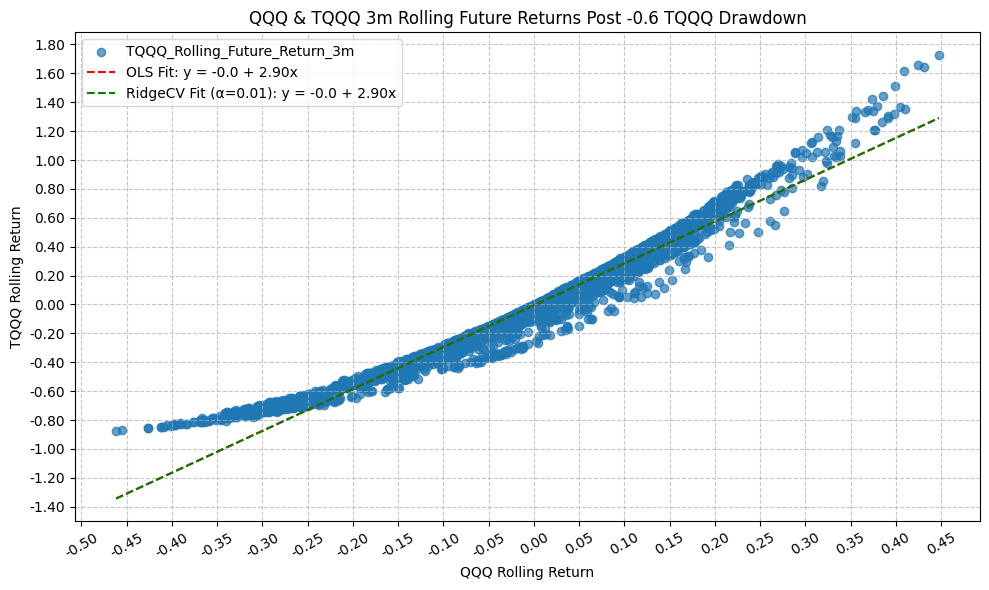
                                  OLS Regression Results
=========================================================================================
Dep. Variable:     TQQQ_Rolling_Future_Return_3m   R-squared:                       0.961
Model:                                       OLS   Adj. R-squared:                  0.961
Method:                            Least Squares   F-statistic:                 1.567e+05
Date:                           Mon, 23 Mar 2026   Prob (F-statistic):               0.00
Time:                                   22:01:03   Log-Likelihood:                 8265.9
No. Observations:                           6281   AIC:                        -1.653e+04
Df Residuals:                               6279   BIC:                        -1.651e+04
Df Model:                                      1
Covariance Type:                       nonrobust
================================================================================================
                                   coef    std err          t      P>|t|      [0.025      0.975]
------------------------------------------------------------------------------------------------
const                           -0.0059      0.001     -7.039      0.000      -0.008      -0.004
QQQ_Rolling_Future_Return_3m     2.8978      0.007    395.792      0.000       2.883       2.912
==============================================================================
Omnibus:                     1352.373   Durbin-Watson:                   0.102
Prob(Omnibus):                  0.000   Jarque-Bera (JB):            15607.922
Skew:                           0.696   Prob(JB):                         0.00
Kurtosis:                      10.596   Cond. No.                         8.95
==============================================================================

Notes:
[1] Standard Errors assume that the covariance matrix of the errors is correctly specified.

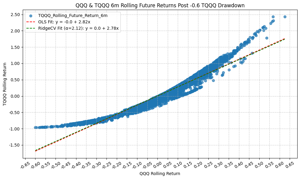
                                  OLS Regression Results
=========================================================================================
Dep. Variable:     TQQQ_Rolling_Future_Return_6m   R-squared:                       0.932
Model:                                       OLS   Adj. R-squared:                  0.932
Method:                            Least Squares   F-statistic:                 8.618e+04
Date:                           Mon, 23 Mar 2026   Prob (F-statistic):               0.00
Time:                                   22:01:05   Log-Likelihood:                 4282.8
No. Observations:                           6281   AIC:                            -8562.
Df Residuals:                               6279   BIC:                            -8548.
Df Model:                                      1
Covariance Type:                       nonrobust
================================================================================================
                                   coef    std err          t      P>|t|      [0.025      0.975]
------------------------------------------------------------------------------------------------
const                           -0.0002      0.002     -0.115      0.909      -0.003       0.003
QQQ_Rolling_Future_Return_6m     2.8190      0.010    293.571      0.000       2.800       2.838
==============================================================================
Omnibus:                     1637.301   Durbin-Watson:                   0.057
Prob(Omnibus):                  0.000   Jarque-Bera (JB):             8392.287
Skew:                           1.158   Prob(JB):                         0.00
Kurtosis:                       8.167   Cond. No.                         6.24
==============================================================================

Notes:
[1] Standard Errors assume that the covariance matrix of the errors is correctly specified.

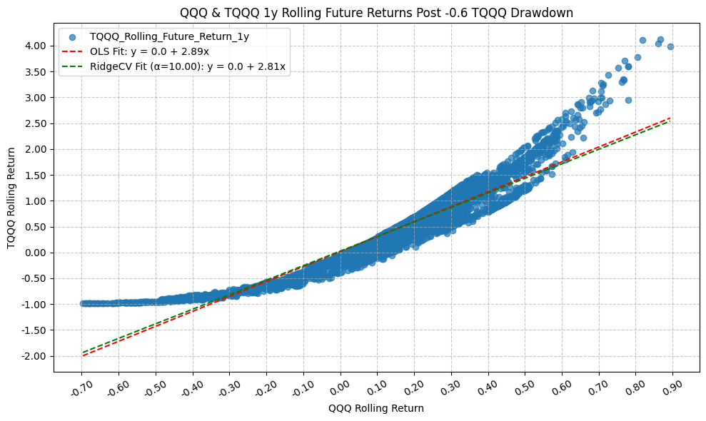
                                  OLS Regression Results
=========================================================================================
Dep. Variable:     TQQQ_Rolling_Future_Return_1y   R-squared:                       0.904
Model:                                       OLS   Adj. R-squared:                  0.904
Method:                            Least Squares   F-statistic:                 5.855e+04
Date:                           Mon, 23 Mar 2026   Prob (F-statistic):               0.00
Time:                                   22:01:07   Log-Likelihood:                 405.83
No. Observations:                           6205   AIC:                            -807.7
Df Residuals:                               6203   BIC:                            -794.2
Df Model:                                      1
Covariance Type:                       nonrobust
================================================================================================
                                   coef    std err          t      P>|t|      [0.025      0.975]
------------------------------------------------------------------------------------------------
const                            0.0161      0.003      4.999      0.000       0.010       0.022
QQQ_Rolling_Future_Return_1y     2.8916      0.012    241.975      0.000       2.868       2.915
==============================================================================
Omnibus:                     1969.830   Durbin-Watson:                   0.038
Prob(Omnibus):                  0.000   Jarque-Bera (JB):             8759.005
Skew:                           1.488   Prob(JB):                         0.00
Kurtosis:                       8.002   Cond. No.                         4.22
==============================================================================

Notes:
[1] Standard Errors assume that the covariance matrix of the errors is correctly specified.
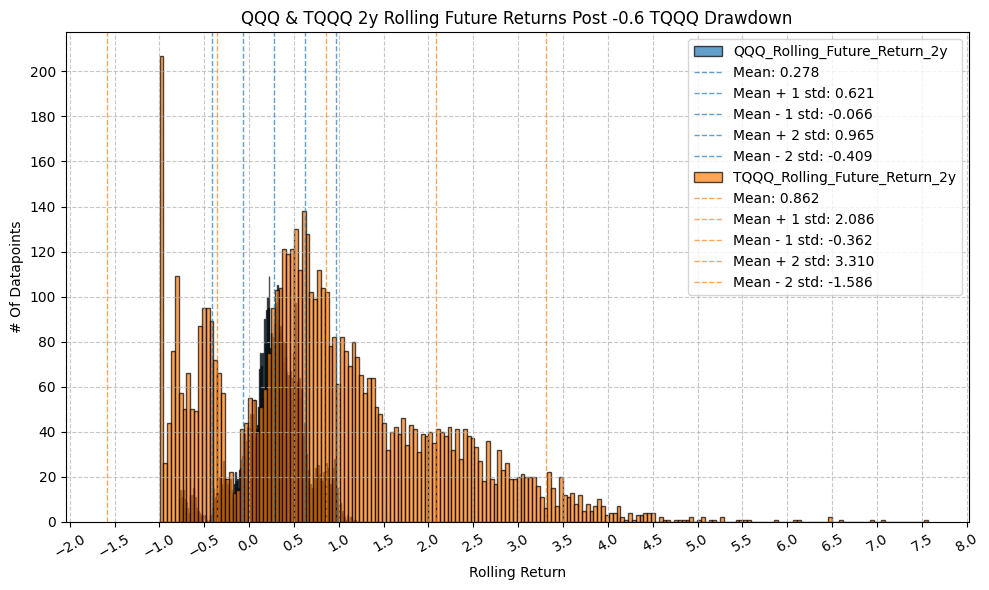

                                  OLS Regression Results
=========================================================================================
Dep. Variable:     TQQQ_Rolling_Future_Return_2y   R-squared:                       0.850
Model:                                       OLS   Adj. R-squared:                  0.850
Method:                            Least Squares   F-statistic:                 3.400e+04
Date:                           Mon, 23 Mar 2026   Prob (F-statistic):               0.00
Time:                                   22:01:09   Log-Likelihood:                -4015.6
No. Observations:                           5983   AIC:                             8035.
Df Residuals:                               5981   BIC:                             8049.
Df Model:                                      1
Covariance Type:                       nonrobust
================================================================================================
                                   coef    std err          t      P>|t|      [0.025      0.975]
------------------------------------------------------------------------------------------------
const                           -0.0508      0.008     -6.452      0.000      -0.066      -0.035
QQQ_Rolling_Future_Return_2y     3.2856      0.018    184.379      0.000       3.251       3.321
==============================================================================
Omnibus:                     1729.276   Durbin-Watson:                   0.019
Prob(Omnibus):                  0.000   Jarque-Bera (JB):             5279.242
Skew:                           1.487   Prob(JB):                         0.00
Kurtosis:                       6.511   Cond. No.                         3.16
==============================================================================

Notes:
[1] Standard Errors assume that the covariance matrix of the errors is correctly specified.
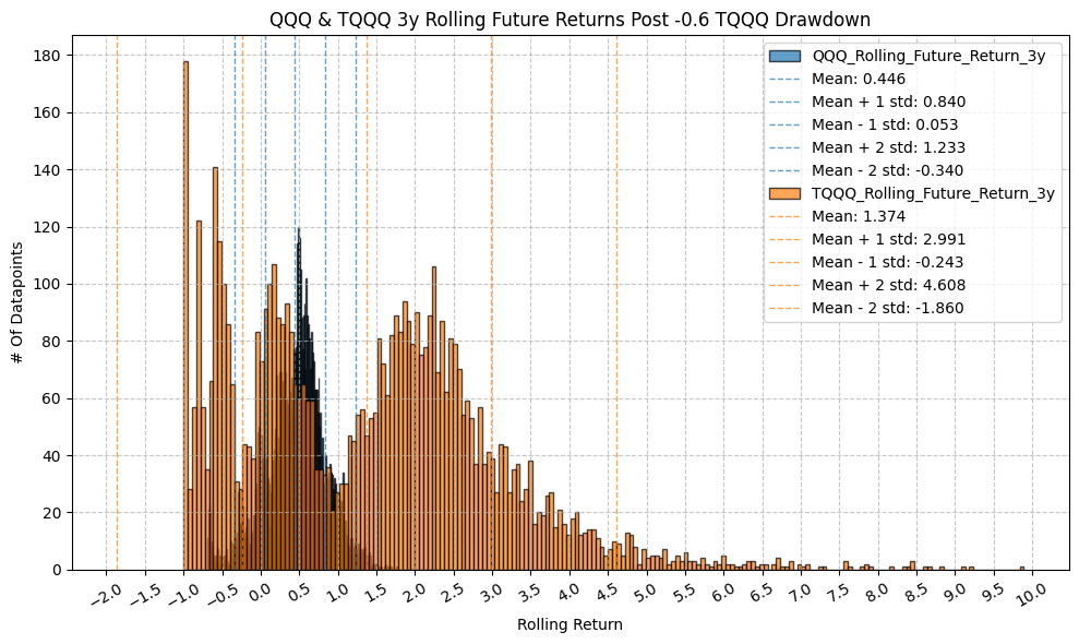

                                  OLS Regression Results
=========================================================================================
Dep. Variable:     TQQQ_Rolling_Future_Return_3y   R-squared:                       0.822
Model:                                       OLS   Adj. R-squared:                  0.821
Method:                            Least Squares   F-statistic:                 2.637e+04
Date:                           Mon, 23 Mar 2026   Prob (F-statistic):               0.00
Time:                                   22:01:11   Log-Likelihood:                -5948.5
No. Observations:                           5731   AIC:                         1.190e+04
Df Residuals:                               5729   BIC:                         1.191e+04
Df Model:                                      1
Covariance Type:                       nonrobust
================================================================================================
                                   coef    std err          t      P>|t|      [0.025      0.975]
------------------------------------------------------------------------------------------------
const                           -0.2891      0.014    -21.177      0.000      -0.316      -0.262
QQQ_Rolling_Future_Return_3y     3.7262      0.023    162.382      0.000       3.681       3.771
==============================================================================
Omnibus:                      849.429   Durbin-Watson:                   0.015
Prob(Omnibus):                  0.000   Jarque-Bera (JB):             1564.767
Skew:                           0.943   Prob(JB):                         0.00
Kurtosis:                       4.731   Cond. No.                         3.12
==============================================================================

Notes:
[1] Standard Errors assume that the covariance matrix of the errors is correctly specified.


                                  OLS Regression Results
=========================================================================================
Dep. Variable:     TQQQ_Rolling_Future_Return_4y   R-squared:                       0.788
Model:                                       OLS   Adj. R-squared:                  0.788
Method:                            Least Squares   F-statistic:                 2.040e+04
Date:                           Mon, 23 Mar 2026   Prob (F-statistic):               0.00
Time:                                   22:01:12   Log-Likelihood:                -8128.7
No. Observations:                           5479   AIC:                         1.626e+04
Df Residuals:                               5477   BIC:                         1.627e+04
Df Model:                                      1
Covariance Type:                       nonrobust
================================================================================================
                                   coef    std err          t      P>|t|      [0.025      0.975]
------------------------------------------------------------------------------------------------
const                           -0.6029      0.024    -25.170      0.000      -0.650      -0.556
QQQ_Rolling_Future_Return_4y     4.3128      0.030    142.830      0.000       4.254       4.372
==============================================================================
Omnibus:                       52.539   Durbin-Watson:                   0.010
Prob(Omnibus):                  0.000   Jarque-Bera (JB):               41.303
Skew:                           0.131   Prob(JB):                     1.07e-09
Kurtosis:                       2.665   Cond. No.                         3.09
==============================================================================

Notes:
[1] Standard Errors assume that the covariance matrix of the errors is correctly specified.

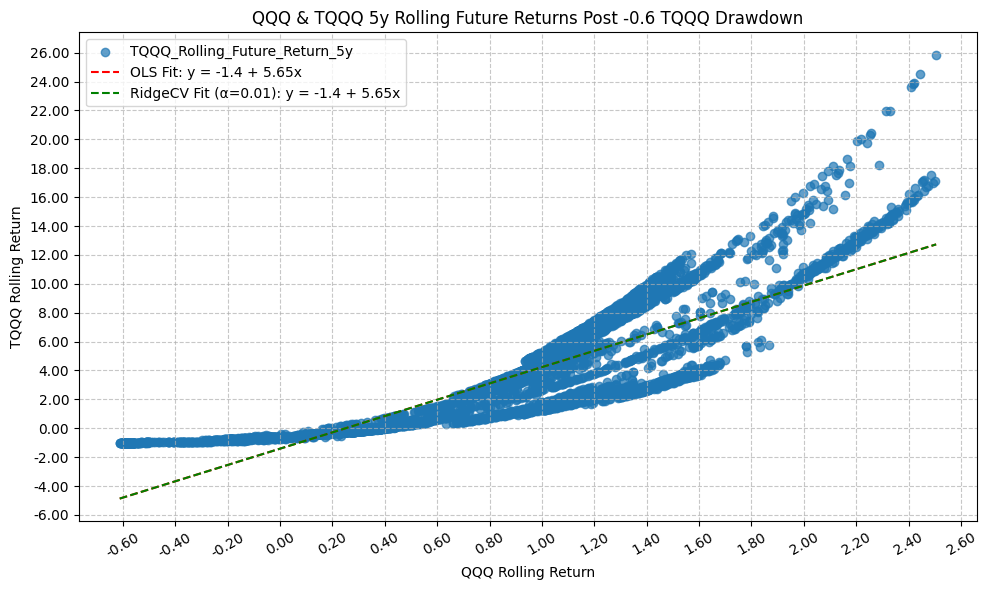
                                  OLS Regression Results
=========================================================================================
Dep. Variable:     TQQQ_Rolling_Future_Return_5y   R-squared:                       0.750
Model:                                       OLS   Adj. R-squared:                  0.750
Method:                            Least Squares   F-statistic:                 1.573e+04
Date:                           Mon, 23 Mar 2026   Prob (F-statistic):               0.00
Time:                                   22:01:14   Log-Likelihood:                -11339.
No. Observations:                           5243   AIC:                         2.268e+04
Df Residuals:                               5241   BIC:                         2.270e+04
Df Model:                                      1
Covariance Type:                       nonrobust
================================================================================================
                                   coef    std err          t      P>|t|      [0.025      0.975]
------------------------------------------------------------------------------------------------
const                           -1.4128      0.050    -28.446      0.000      -1.510      -1.315
QQQ_Rolling_Future_Return_5y     5.6452      0.045    125.418      0.000       5.557       5.733
==============================================================================
Omnibus:                      227.541   Durbin-Watson:                   0.009
Prob(Omnibus):                  0.000   Jarque-Bera (JB):              348.386
Skew:                           0.394   Prob(JB):                     2.23e-76
Kurtosis:                       3.988   Cond. No.                         3.11
==============================================================================

Notes:
[1] Standard Errors assume that the covariance matrix of the errors is correctly specified.


                                  OLS Regression Results
=========================================================================================
Dep. Variable:     TQQQ_Rolling_Future_Return_1d   R-squared:                       0.999
Model:                                       OLS   Adj. R-squared:                  0.999
Method:                            Least Squares   F-statistic:                 5.380e+06
Date:                           Mon, 23 Mar 2026   Prob (F-statistic):               0.00
Time:                                   22:01:16   Log-Likelihood:                 29443.
No. Observations:                           5890   AIC:                        -5.888e+04
Df Residuals:                               5888   BIC:                        -5.887e+04
Df Model:                                      1
Covariance Type:                       nonrobust
================================================================================================
                                   coef    std err          t      P>|t|      [0.025      0.975]
------------------------------------------------------------------------------------------------
const                        -3.037e-05   2.13e-05     -1.427      0.154   -7.21e-05    1.14e-05
QQQ_Rolling_Future_Return_1d     2.9544      0.001   2319.390      0.000       2.952       2.957
==============================================================================
Omnibus:                     8698.998   Durbin-Watson:                   2.576
Prob(Omnibus):                  0.000   Jarque-Bera (JB):         31790538.925
Skew:                          -8.045   Prob(JB):                         0.00
Kurtosis:                     362.553   Cond. No.                         59.9
==============================================================================

Notes:
[1] Standard Errors assume that the covariance matrix of the errors is correctly specified.


                                  OLS Regression Results
=========================================================================================
Dep. Variable:     TQQQ_Rolling_Future_Return_1w   R-squared:                       0.994
Model:                                       OLS   Adj. R-squared:                  0.994
Method:                            Least Squares   F-statistic:                 1.008e+06
Date:                           Mon, 23 Mar 2026   Prob (F-statistic):               0.00
Time:                                   22:01:18   Log-Likelihood:                 20303.
No. Observations:                           5890   AIC:                        -4.060e+04
Df Residuals:                               5888   BIC:                        -4.059e+04
Df Model:                                      1
Covariance Type:                       nonrobust
================================================================================================
                                   coef    std err          t      P>|t|      [0.025      0.975]
------------------------------------------------------------------------------------------------
const                           -0.0006      0.000     -6.363      0.000      -0.001      -0.000
QQQ_Rolling_Future_Return_1w     2.9526      0.003   1003.859      0.000       2.947       2.958
==============================================================================
Omnibus:                     3288.219   Durbin-Watson:                   0.897
Prob(Omnibus):                  0.000   Jarque-Bera (JB):           369148.693
Skew:                          -1.720   Prob(JB):                         0.00
Kurtosis:                      41.631   Cond. No.                         29.3
==============================================================================

Notes:
[1] Standard Errors assume that the covariance matrix of the errors is correctly specified.


                                  OLS Regression Results
=========================================================================================
Dep. Variable:     TQQQ_Rolling_Future_Return_1m   R-squared:                       0.983
Model:                                       OLS   Adj. R-squared:                  0.983
Method:                            Least Squares   F-statistic:                 3.372e+05
Date:                           Mon, 23 Mar 2026   Prob (F-statistic):               0.00
Time:                                   22:01:20   Log-Likelihood:                 13210.
No. Observations:                           5890   AIC:                        -2.642e+04
Df Residuals:                               5888   BIC:                        -2.640e+04
Df Model:                                      1
Covariance Type:                       nonrobust
================================================================================================
                                   coef    std err          t      P>|t|      [0.025      0.975]
------------------------------------------------------------------------------------------------
const                           -0.0025      0.000     -7.379      0.000      -0.003      -0.002
QQQ_Rolling_Future_Return_1m     2.9140      0.005    580.676      0.000       2.904       2.924
==============================================================================
Omnibus:                     1415.341   Durbin-Watson:                   0.310
Prob(Omnibus):                  0.000   Jarque-Bera (JB):            78303.043
Skew:                           0.193   Prob(JB):                         0.00
Kurtosis:                      20.858   Cond. No.                         15.0
==============================================================================

Notes:
[1] Standard Errors assume that the covariance matrix of the errors is correctly specified.
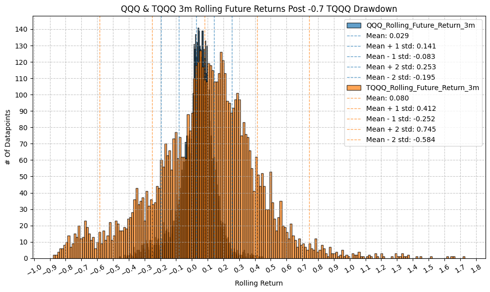

                                  OLS Regression Results
=========================================================================================
Dep. Variable:     TQQQ_Rolling_Future_Return_3m   R-squared:                       0.962
Model:                                       OLS   Adj. R-squared:                  0.962
Method:                            Least Squares   F-statistic:                 1.509e+05
Date:                           Mon, 23 Mar 2026   Prob (F-statistic):               0.00
Time:                                   22:01:21   Log-Likelihood:                 7799.8
No. Observations:                           5890   AIC:                        -1.560e+04
Df Residuals:                               5888   BIC:                        -1.558e+04
Df Model:                                      1
Covariance Type:                       nonrobust
================================================================================================
                                   coef    std err          t      P>|t|      [0.025      0.975]
------------------------------------------------------------------------------------------------
const                           -0.0040      0.001     -4.619      0.000      -0.006      -0.002
QQQ_Rolling_Future_Return_3m     2.9068      0.007    388.462      0.000       2.892       2.921
==============================================================================
Omnibus:                     1368.479   Durbin-Watson:                   0.107
Prob(Omnibus):                  0.000   Jarque-Bera (JB):            16451.791
Skew:                           0.766   Prob(JB):                         0.00
Kurtosis:                      11.043   Cond. No.                         8.93
==============================================================================

Notes:
[1] Standard Errors assume that the covariance matrix of the errors is correctly specified.
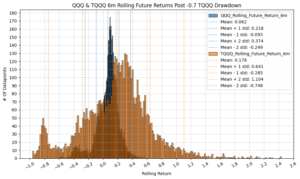

                                  OLS Regression Results
=========================================================================================
Dep. Variable:     TQQQ_Rolling_Future_Return_6m   R-squared:                       0.934
Model:                                       OLS   Adj. R-squared:                  0.934
Method:                            Least Squares   F-statistic:                 8.379e+04
Date:                           Mon, 23 Mar 2026   Prob (F-statistic):               0.00
Time:                                   22:01:23   Log-Likelihood:                 4198.8
No. Observations:                           5890   AIC:                            -8394.
Df Residuals:                               5888   BIC:                            -8380.
Df Model:                                      1
Covariance Type:                       nonrobust
================================================================================================
                                   coef    std err          t      P>|t|      [0.025      0.975]
------------------------------------------------------------------------------------------------
const                           -0.0018      0.002     -1.052      0.293      -0.005       0.002
QQQ_Rolling_Future_Return_6m     2.8731      0.010    289.460      0.000       2.854       2.893
==============================================================================
Omnibus:                     1462.376   Durbin-Watson:                   0.063
Prob(Omnibus):                  0.000   Jarque-Bera (JB):             8112.635
Skew:                           1.074   Prob(JB):                         0.00
Kurtosis:                       8.333   Cond. No.                         6.45
==============================================================================

Notes:
[1] Standard Errors assume that the covariance matrix of the errors is correctly specified.
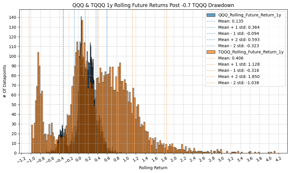
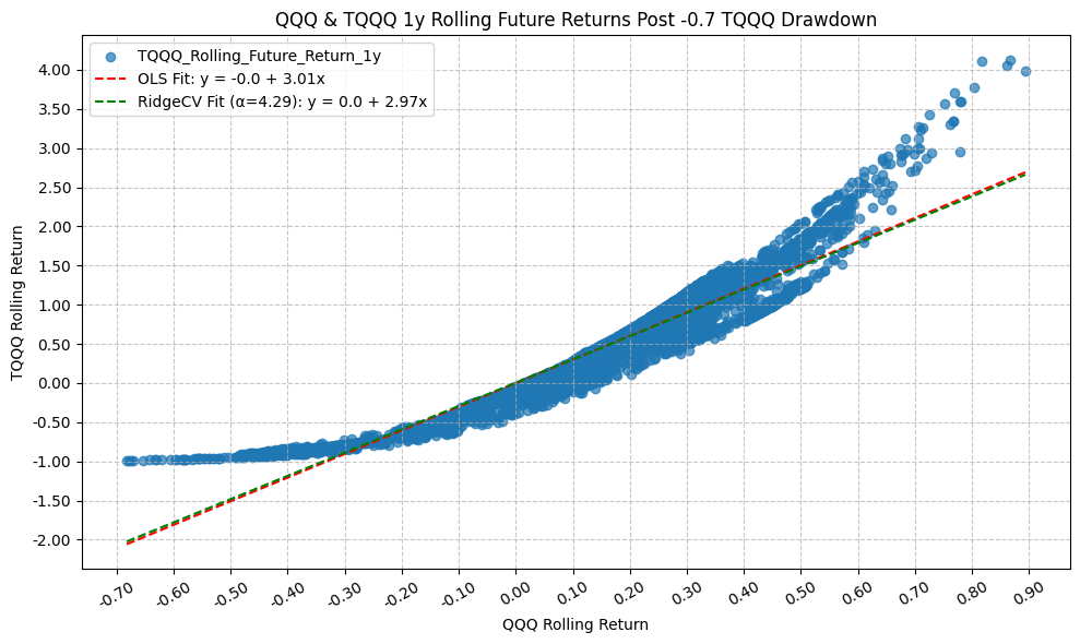
                                  OLS Regression Results
=========================================================================================
Dep. Variable:     TQQQ_Rolling_Future_Return_1y   R-squared:                       0.912
Model:                                       OLS   Adj. R-squared:                  0.912
Method:                            Least Squares   F-statistic:                 6.072e+04
Date:                           Mon, 23 Mar 2026   Prob (F-statistic):               0.00
Time:                                   22:01:25   Log-Likelihood:                 715.42
No. Observations:                           5857   AIC:                            -1427.
Df Residuals:                               5855   BIC:                            -1413.
Df Model:                                      1
Covariance Type:                       nonrobust
================================================================================================
                                   coef    std err          t      P>|t|      [0.025      0.975]
------------------------------------------------------------------------------------------------
const                           -0.0011      0.003     -0.327      0.744      -0.007       0.005
QQQ_Rolling_Future_Return_1y     3.0129      0.012    246.405      0.000       2.989       3.037
==============================================================================
Omnibus:                     1765.613   Durbin-Watson:                   0.043
Prob(Omnibus):                  0.000   Jarque-Bera (JB):             8325.388
Skew:                           1.385   Prob(JB):                         0.00
Kurtosis:                       8.142   Cond. No.                         4.45
==============================================================================

Notes:
[1] Standard Errors assume that the covariance matrix of the errors is correctly specified.
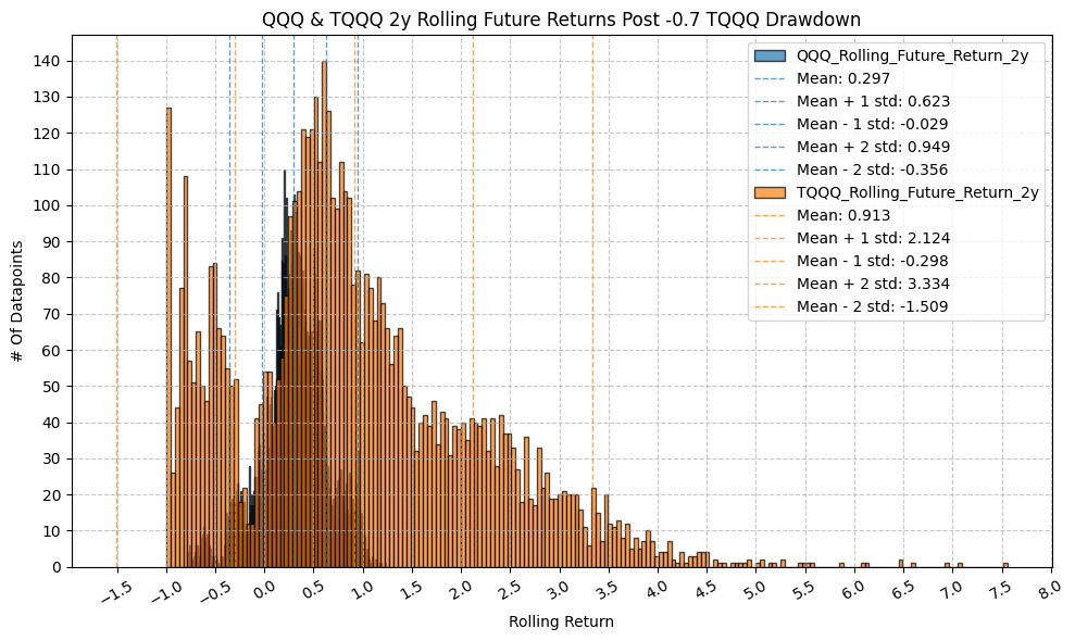
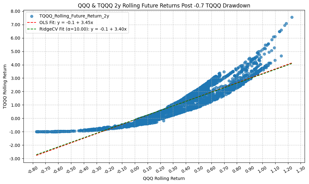
                                  OLS Regression Results
=========================================================================================
Dep. Variable:     TQQQ_Rolling_Future_Return_2y   R-squared:                       0.865
Model:                                       OLS   Adj. R-squared:                  0.865
Method:                            Least Squares   F-statistic:                 3.711e+04
Date:                           Mon, 23 Mar 2026   Prob (F-statistic):               0.00
Time:                                   22:01:27   Log-Likelihood:                -3522.7
No. Observations:                           5789   AIC:                             7049.
Df Residuals:                               5787   BIC:                             7063.
Df Model:                                      1
Covariance Type:                       nonrobust
================================================================================================
                                   coef    std err          t      P>|t|      [0.025      0.975]
------------------------------------------------------------------------------------------------
const                           -0.1121      0.008    -14.185      0.000      -0.128      -0.097
QQQ_Rolling_Future_Return_2y     3.4520      0.018    192.643      0.000       3.417       3.487
==============================================================================
Omnibus:                     1654.985   Durbin-Watson:                   0.020
Prob(Omnibus):                  0.000   Jarque-Bera (JB):             5614.089
Skew:                           1.426   Prob(JB):                         0.00
Kurtosis:                       6.891   Cond. No.                         3.36
==============================================================================

Notes:
[1] Standard Errors assume that the covariance matrix of the errors is correctly specified.
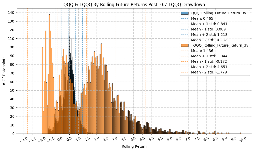

                                  OLS Regression Results
=========================================================================================
Dep. Variable:     TQQQ_Rolling_Future_Return_3y   R-squared:                       0.838
Model:                                       OLS   Adj. R-squared:                  0.838
Method:                            Least Squares   F-statistic:                 2.860e+04
Date:                           Mon, 23 Mar 2026   Prob (F-statistic):               0.00
Time:                                   22:01:28   Log-Likelihood:                -5448.4
No. Observations:                           5537   AIC:                         1.090e+04
Df Residuals:                               5535   BIC:                         1.091e+04
Df Model:                                      1
Covariance Type:                       nonrobust
================================================================================================
                                   coef    std err          t      P>|t|      [0.025      0.975]
------------------------------------------------------------------------------------------------
const                           -0.3842      0.014    -27.758      0.000      -0.411      -0.357
QQQ_Rolling_Future_Return_3y     3.9118      0.023    169.113      0.000       3.866       3.957
==============================================================================
Omnibus:                      674.134   Durbin-Watson:                   0.016
Prob(Omnibus):                  0.000   Jarque-Bera (JB):             1252.709
Skew:                           0.794   Prob(JB):                    9.50e-273
Kurtosis:                       4.706   Cond. No.                         3.31
==============================================================================

Notes:
[1] Standard Errors assume that the covariance matrix of the errors is correctly specified.
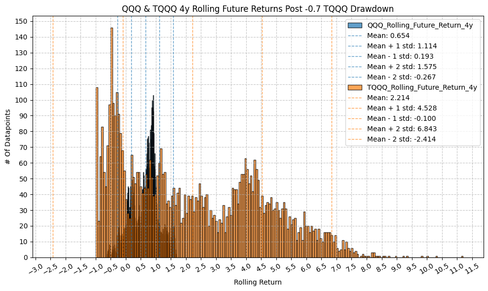
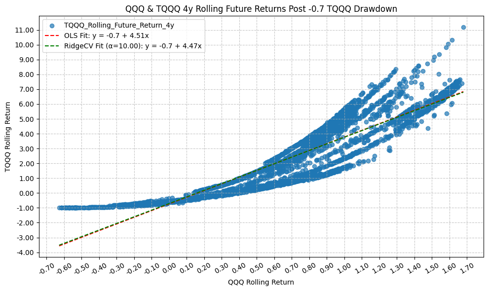
                                  OLS Regression Results
=========================================================================================
Dep. Variable:     TQQQ_Rolling_Future_Return_4y   R-squared:                       0.805
Model:                                       OLS   Adj. R-squared:                  0.805
Method:                            Least Squares   F-statistic:                 2.185e+04
Date:                           Mon, 23 Mar 2026   Prob (F-statistic):               0.00
Time:                                   22:01:30   Log-Likelihood:                -7609.7
No. Observations:                           5285   AIC:                         1.522e+04
Df Residuals:                               5283   BIC:                         1.524e+04
Df Model:                                      1
Covariance Type:                       nonrobust
================================================================================================
                                   coef    std err          t      P>|t|      [0.025      0.975]
------------------------------------------------------------------------------------------------
const                           -0.7332      0.024    -30.056      0.000      -0.781      -0.685
QQQ_Rolling_Future_Return_4y     4.5096      0.031    147.803      0.000       4.450       4.569
==============================================================================
Omnibus:                       12.958   Durbin-Watson:                   0.011
Prob(Omnibus):                  0.002   Jarque-Bera (JB):               10.506
Skew:                          -0.007   Prob(JB):                      0.00523
Kurtosis:                       2.782   Cond. No.                         3.25
==============================================================================

Notes:
[1] Standard Errors assume that the covariance matrix of the errors is correctly specified.

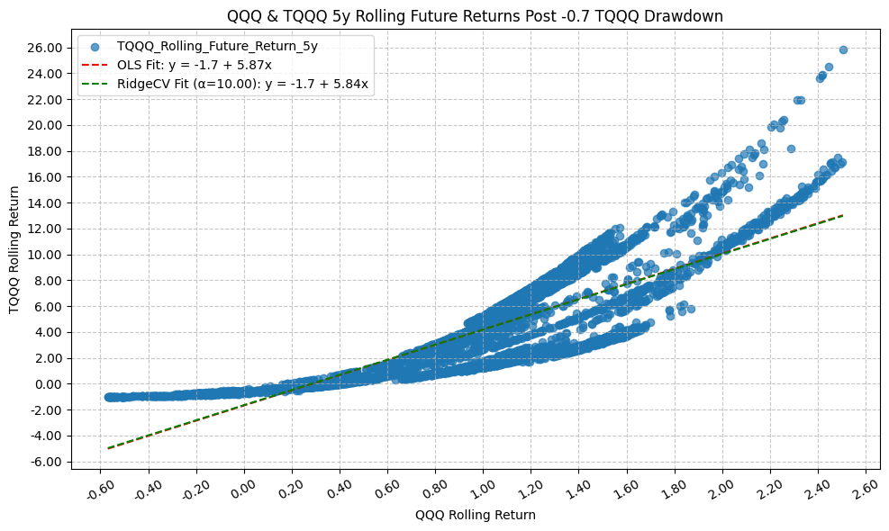
                                  OLS Regression Results
=========================================================================================
Dep. Variable:     TQQQ_Rolling_Future_Return_5y   R-squared:                       0.759
Model:                                       OLS   Adj. R-squared:                  0.759
Method:                            Least Squares   F-statistic:                 1.625e+04
Date:                           Mon, 23 Mar 2026   Prob (F-statistic):               0.00
Time:                                   22:01:32   Log-Likelihood:                -11064.
No. Observations:                           5163   AIC:                         2.213e+04
Df Residuals:                               5161   BIC:                         2.215e+04
Df Model:                                      1
Covariance Type:                       nonrobust
================================================================================================
                                   coef    std err          t      P>|t|      [0.025      0.975]
------------------------------------------------------------------------------------------------
const                           -1.6771      0.051    -32.821      0.000      -1.777      -1.577
QQQ_Rolling_Future_Return_5y     5.8699      0.046    127.459      0.000       5.780       5.960
==============================================================================
Omnibus:                      168.793   Durbin-Watson:                   0.010
Prob(Omnibus):                  0.000   Jarque-Bera (JB):              286.855
Skew:                           0.283   Prob(JB):                     5.13e-63
Kurtosis:                       4.007   Cond. No.                         3.27
==============================================================================

Notes:
[1] Standard Errors assume that the covariance matrix of the errors is correctly specified.


                                  OLS Regression Results
=========================================================================================
Dep. Variable:     TQQQ_Rolling_Future_Return_1d   R-squared:                       0.999
Model:                                       OLS   Adj. R-squared:                  0.999
Method:                            Least Squares   F-statistic:                 4.767e+06
Date:                           Mon, 23 Mar 2026   Prob (F-statistic):               0.00
Time:                                   22:01:33   Log-Likelihood:                 27167.
No. Observations:                           5450   AIC:                        -5.433e+04
Df Residuals:                               5448   BIC:                        -5.432e+04
Df Model:                                      1
Covariance Type:                       nonrobust
================================================================================================
                                   coef    std err          t      P>|t|      [0.025      0.975]
------------------------------------------------------------------------------------------------
const                        -1.602e-05   2.24e-05     -0.714      0.475      -6e-05     2.8e-05
QQQ_Rolling_Future_Return_1d     2.9532      0.001   2183.311      0.000       2.951       2.956
==============================================================================
Omnibus:                     8184.121   Durbin-Watson:                   2.578
Prob(Omnibus):                  0.000   Jarque-Bera (JB):         30349901.921
Skew:                          -8.326   Prob(JB):                         0.00
Kurtosis:                     368.204   Cond. No.                         60.3
==============================================================================

Notes:
[1] Standard Errors assume that the covariance matrix of the errors is correctly specified.
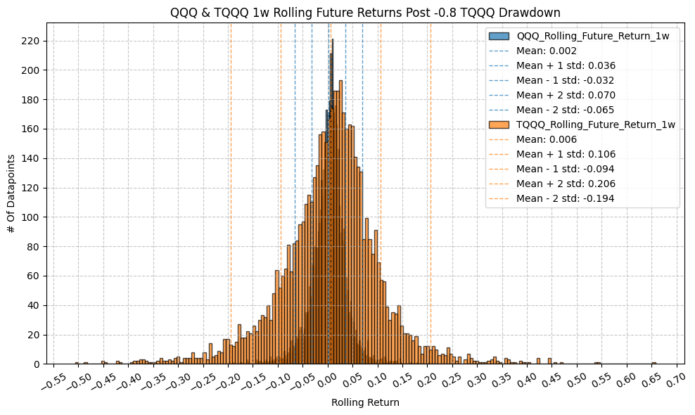

                                  OLS Regression Results
=========================================================================================
Dep. Variable:     TQQQ_Rolling_Future_Return_1w   R-squared:                       0.994
Model:                                       OLS   Adj. R-squared:                  0.994
Method:                            Least Squares   F-statistic:                 9.352e+05
Date:                           Mon, 23 Mar 2026   Prob (F-statistic):               0.00
Time:                                   22:01:35   Log-Likelihood:                 18855.
No. Observations:                           5450   AIC:                        -3.771e+04
Df Residuals:                               5448   BIC:                        -3.769e+04
Df Model:                                      1
Covariance Type:                       nonrobust
================================================================================================
                                   coef    std err          t      P>|t|      [0.025      0.975]
------------------------------------------------------------------------------------------------
const                           -0.0006      0.000     -5.512      0.000      -0.001      -0.000
QQQ_Rolling_Future_Return_1w     2.9495      0.003    967.071      0.000       2.944       2.956
==============================================================================
Omnibus:                     3225.262   Durbin-Watson:                   0.872
Prob(Omnibus):                  0.000   Jarque-Bera (JB):           383451.023
Skew:                          -1.880   Prob(JB):                         0.00
Kurtosis:                      43.920   Cond. No.                         29.6
==============================================================================

Notes:
[1] Standard Errors assume that the covariance matrix of the errors is correctly specified.

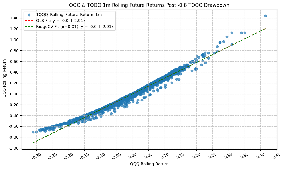
                                  OLS Regression Results
=========================================================================================
Dep. Variable:     TQQQ_Rolling_Future_Return_1m   R-squared:                       0.982
Model:                                       OLS   Adj. R-squared:                  0.982
Method:                            Least Squares   F-statistic:                 3.035e+05
Date:                           Mon, 23 Mar 2026   Prob (F-statistic):               0.00
Time:                                   22:01:37   Log-Likelihood:                 12190.
No. Observations:                           5450   AIC:                        -2.438e+04
Df Residuals:                               5448   BIC:                        -2.436e+04
Df Model:                                      1
Covariance Type:                       nonrobust
================================================================================================
                                   coef    std err          t      P>|t|      [0.025      0.975]
------------------------------------------------------------------------------------------------
const                           -0.0021      0.000     -5.911      0.000      -0.003      -0.001
QQQ_Rolling_Future_Return_1m     2.9063      0.005    550.932      0.000       2.896       2.917
==============================================================================
Omnibus:                     1331.250   Durbin-Watson:                   0.299
Prob(Omnibus):                  0.000   Jarque-Bera (JB):            76809.720
Skew:                           0.205   Prob(JB):                         0.00
Kurtosis:                      21.387   Cond. No.                         15.1
==============================================================================

Notes:
[1] Standard Errors assume that the covariance matrix of the errors is correctly specified.
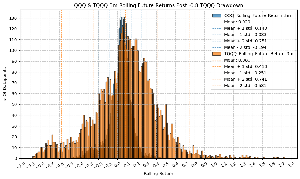
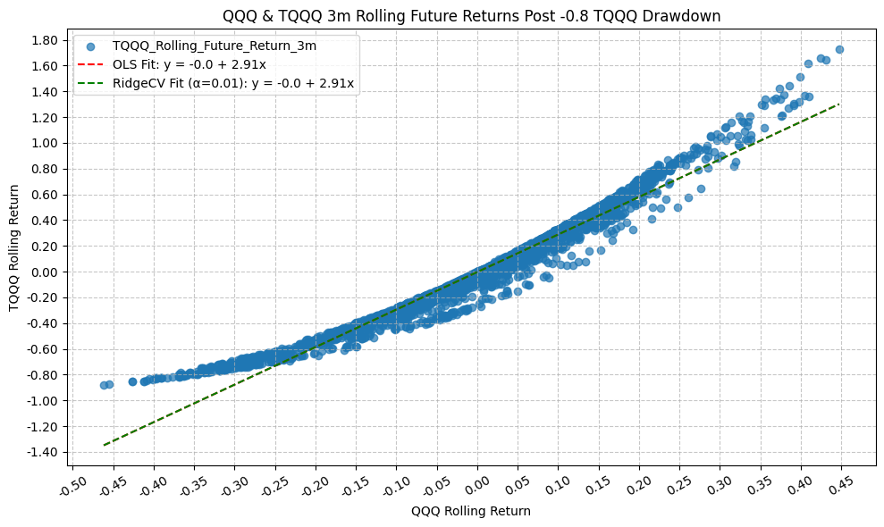
                                  OLS Regression Results
=========================================================================================
Dep. Variable:     TQQQ_Rolling_Future_Return_3m   R-squared:                       0.961
Model:                                       OLS   Adj. R-squared:                  0.961
Method:                            Least Squares   F-statistic:                 1.352e+05
Date:                           Mon, 23 Mar 2026   Prob (F-statistic):               0.00
Time:                                   22:01:38   Log-Likelihood:                 7159.6
No. Observations:                           5450   AIC:                        -1.432e+04
Df Residuals:                               5448   BIC:                        -1.430e+04
Df Model:                                      1
Covariance Type:                       nonrobust
================================================================================================
                                   coef    std err          t      P>|t|      [0.025      0.975]
------------------------------------------------------------------------------------------------
const                           -0.0036      0.001     -3.910      0.000      -0.005      -0.002
QQQ_Rolling_Future_Return_3m     2.9142      0.008    367.681      0.000       2.899       2.930
==============================================================================
Omnibus:                     1265.130   Durbin-Watson:                   0.097
Prob(Omnibus):                  0.000   Jarque-Bera (JB):            15817.100
Skew:                           0.752   Prob(JB):                         0.00
Kurtosis:                      11.209   Cond. No.                         9.00
==============================================================================

Notes:
[1] Standard Errors assume that the covariance matrix of the errors is correctly specified.
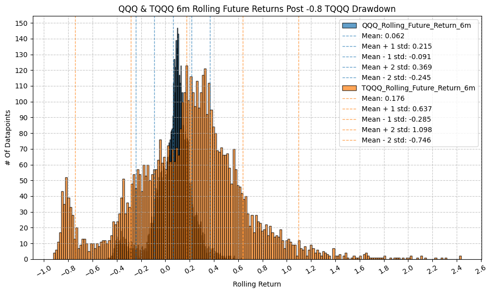
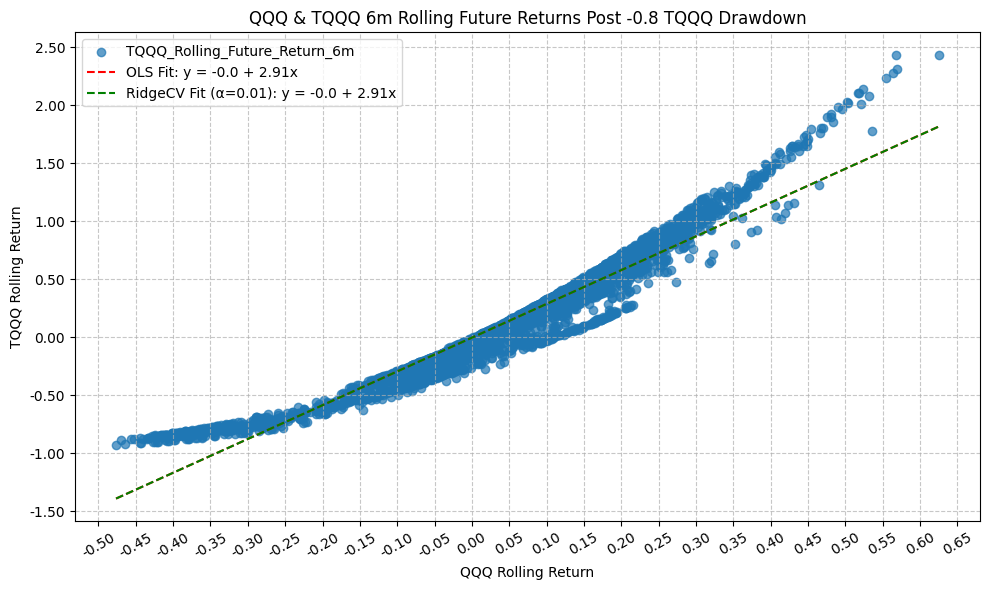
                                  OLS Regression Results
=========================================================================================
Dep. Variable:     TQQQ_Rolling_Future_Return_6m   R-squared:                       0.937
Model:                                       OLS   Adj. R-squared:                  0.937
Method:                            Least Squares   F-statistic:                 8.117e+04
Date:                           Mon, 23 Mar 2026   Prob (F-statistic):               0.00
Time:                                   22:01:40   Log-Likelihood:                 4027.1
No. Observations:                           5450   AIC:                            -8050.
Df Residuals:                               5448   BIC:                            -8037.
Df Model:                                      1
Covariance Type:                       nonrobust
================================================================================================
                                   coef    std err          t      P>|t|      [0.025      0.975]
------------------------------------------------------------------------------------------------
const                           -0.0043      0.002     -2.531      0.011      -0.008      -0.001
QQQ_Rolling_Future_Return_6m     2.9104      0.010    284.899      0.000       2.890       2.930
==============================================================================
Omnibus:                      970.645   Durbin-Watson:                   0.061
Prob(Omnibus):                  0.000   Jarque-Bera (JB):             4546.797
Skew:                           0.789   Prob(JB):                         0.00
Kurtosis:                       7.187   Cond. No.                         6.55
==============================================================================

Notes:
[1] Standard Errors assume that the covariance matrix of the errors is correctly specified.
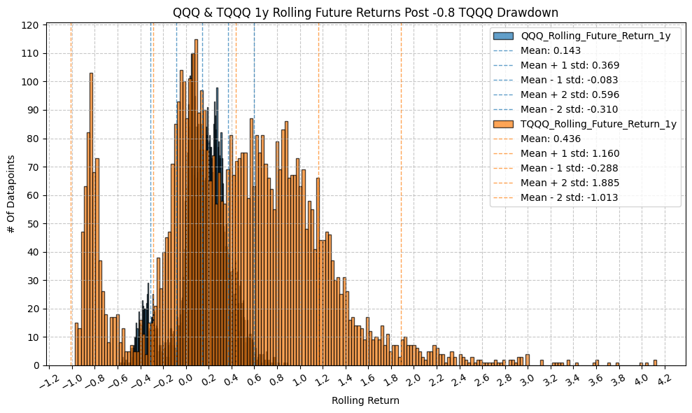
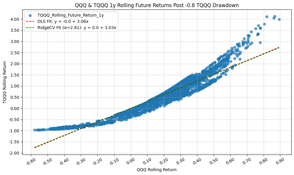
                                  OLS Regression Results
=========================================================================================
Dep. Variable:     TQQQ_Rolling_Future_Return_1y   R-squared:                       0.917
Model:                                       OLS   Adj. R-squared:                  0.917
Method:                            Least Squares   F-statistic:                 5.979e+04
Date:                           Mon, 23 Mar 2026   Prob (F-statistic):               0.00
Time:                                   22:01:42   Log-Likelihood:                 790.67
No. Observations:                           5446   AIC:                            -1577.
Df Residuals:                               5444   BIC:                            -1564.
Df Model:                                      1
Covariance Type:                       nonrobust
================================================================================================
                                   coef    std err          t      P>|t|      [0.025      0.975]
------------------------------------------------------------------------------------------------
const                           -0.0019      0.003     -0.560      0.575      -0.008       0.005
QQQ_Rolling_Future_Return_1y     3.0627      0.013    244.513      0.000       3.038       3.087
==============================================================================
Omnibus:                     1401.338   Durbin-Watson:                   0.045
Prob(Omnibus):                  0.000   Jarque-Bera (JB):             6208.882
Skew:                           1.187   Prob(JB):                         0.00
Kurtosis:                       7.661   Cond. No.                         4.51
==============================================================================

Notes:
[1] Standard Errors assume that the covariance matrix of the errors is correctly specified.
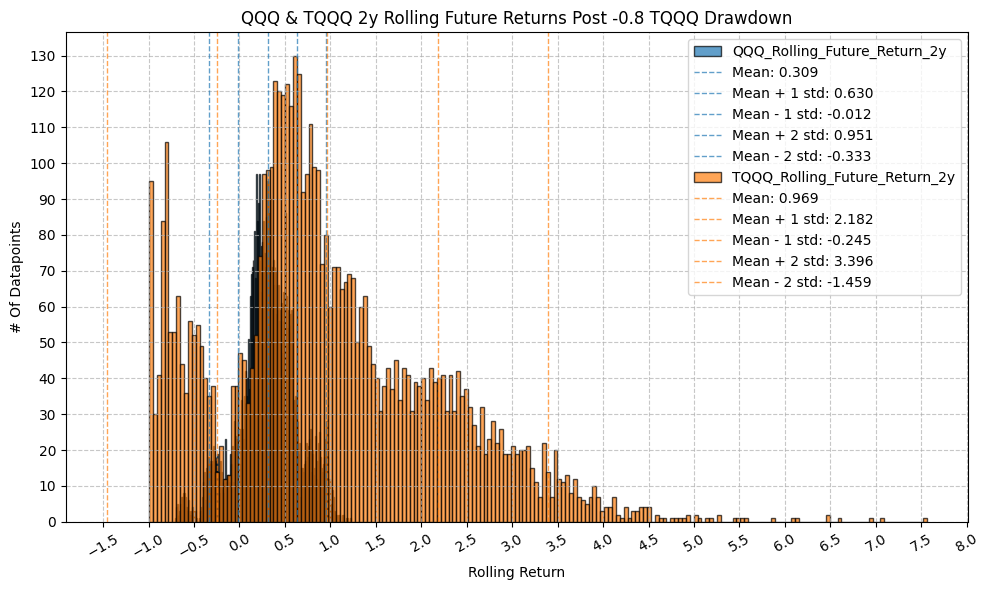
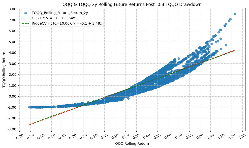
                                  OLS Regression Results
=========================================================================================
Dep. Variable:     TQQQ_Rolling_Future_Return_2y   R-squared:                       0.876
Model:                                       OLS   Adj. R-squared:                  0.876
Method:                            Least Squares   F-statistic:                 3.834e+04
Date:                           Mon, 23 Mar 2026   Prob (F-statistic):               0.00
Time:                                   22:01:43   Log-Likelihood:                -3105.2
No. Observations:                           5446   AIC:                             6214.
Df Residuals:                               5444   BIC:                             6228.
Df Model:                                      1
Covariance Type:                       nonrobust
================================================================================================
                                   coef    std err          t      P>|t|      [0.025      0.975]
------------------------------------------------------------------------------------------------
const                           -0.1258      0.008    -15.614      0.000      -0.142      -0.110
QQQ_Rolling_Future_Return_2y     3.5394      0.018    195.794      0.000       3.504       3.575
==============================================================================
Omnibus:                     1479.606   Durbin-Watson:                   0.022
Prob(Omnibus):                  0.000   Jarque-Bera (JB):             5093.275
Skew:                           1.346   Prob(JB):                         0.00
Kurtosis:                       6.899   Cond. No.                         3.45
==============================================================================

Notes:
[1] Standard Errors assume that the covariance matrix of the errors is correctly specified.
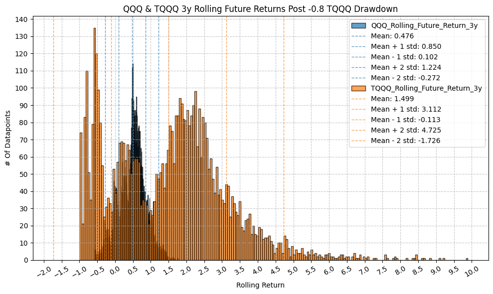
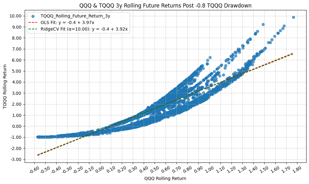
                                  OLS Regression Results
=========================================================================================
Dep. Variable:     TQQQ_Rolling_Future_Return_3y   R-squared:                       0.850
Model:                                       OLS   Adj. R-squared:                  0.850
Method:                            Least Squares   F-statistic:                 2.993e+04
Date:                           Mon, 23 Mar 2026   Prob (F-statistic):               0.00
Time:                                   22:01:45   Log-Likelihood:                -5026.2
No. Observations:                           5295   AIC:                         1.006e+04
Df Residuals:                               5293   BIC:                         1.007e+04
Df Model:                                      1
Covariance Type:                       nonrobust
================================================================================================
                                   coef    std err          t      P>|t|      [0.025      0.975]
------------------------------------------------------------------------------------------------
const                           -0.3931      0.014    -28.257      0.000      -0.420      -0.366
QQQ_Rolling_Future_Return_3y     3.9740      0.023    172.992      0.000       3.929       4.019
==============================================================================
Omnibus:                      582.216   Durbin-Watson:                   0.018
Prob(Omnibus):                  0.000   Jarque-Bera (JB):             1156.163
Skew:                           0.707   Prob(JB):                    8.76e-252
Kurtosis:                       4.801   Cond. No.                         3.36
==============================================================================

Notes:
[1] Standard Errors assume that the covariance matrix of the errors is correctly specified.
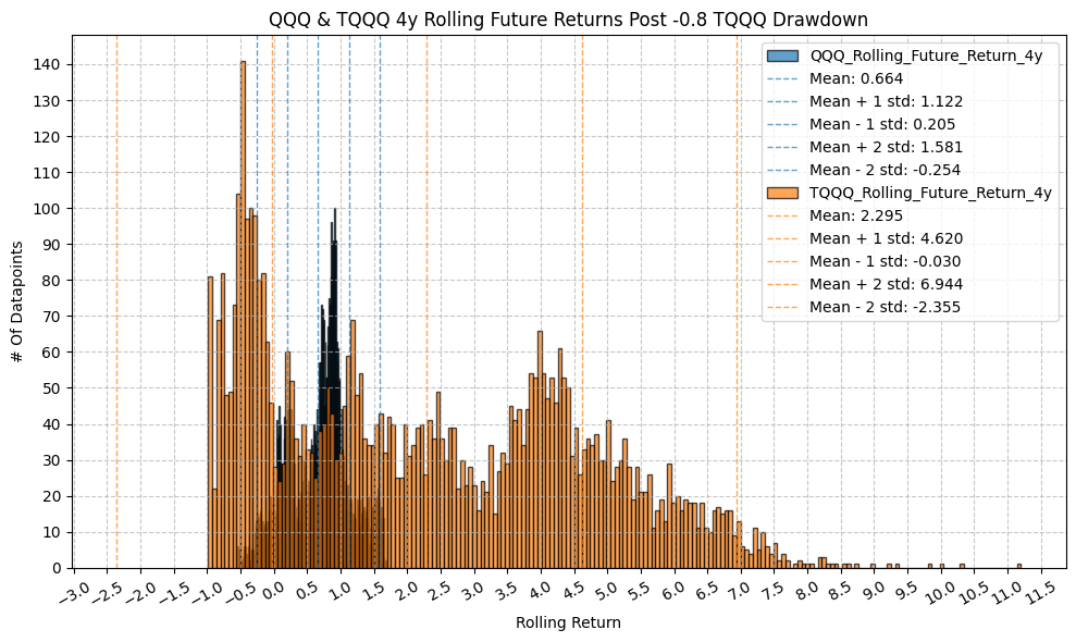
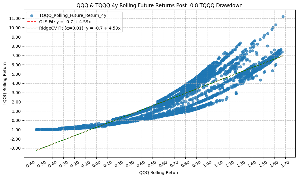
                                  OLS Regression Results
=========================================================================================
Dep. Variable:     TQQQ_Rolling_Future_Return_4y   R-squared:                       0.819
Model:                                       OLS   Adj. R-squared:                  0.819
Method:                            Least Squares   F-statistic:                 2.300e+04
Date:                           Mon, 23 Mar 2026   Prob (F-statistic):               0.00
Time:                                   22:01:47   Log-Likelihood:                -7134.0
No. Observations:                           5071   AIC:                         1.427e+04
Df Residuals:                               5069   BIC:                         1.429e+04
Df Model:                                      1
Covariance Type:                       nonrobust
================================================================================================
                                   coef    std err          t      P>|t|      [0.025      0.975]
------------------------------------------------------------------------------------------------
const                           -0.7493      0.024    -30.704      0.000      -0.797      -0.701
QQQ_Rolling_Future_Return_4y     4.5868      0.030    151.643      0.000       4.528       4.646
==============================================================================
Omnibus:                       13.206   Durbin-Watson:                   0.011
Prob(Omnibus):                  0.001   Jarque-Bera (JB):               13.284
Skew:                          -0.121   Prob(JB):                      0.00130
Kurtosis:                       2.931   Cond. No.                         3.30
==============================================================================

Notes:
[1] Standard Errors assume that the covariance matrix of the errors is correctly specified.


                                  OLS Regression Results
=========================================================================================
Dep. Variable:     TQQQ_Rolling_Future_Return_5y   R-squared:                       0.766
Model:                                       OLS   Adj. R-squared:                  0.766
Method:                            Least Squares   F-statistic:                 1.658e+04
Date:                           Mon, 23 Mar 2026   Prob (F-statistic):               0.00
Time:                                   22:01:48   Log-Likelihood:                -10802.
No. Observations:                           5069   AIC:                         2.161e+04
Df Residuals:                               5067   BIC:                         2.162e+04
Df Model:                                      1
Covariance Type:                       nonrobust
================================================================================================
                                   coef    std err          t      P>|t|      [0.025      0.975]
------------------------------------------------------------------------------------------------
const                           -1.7617      0.052    -34.121      0.000      -1.863      -1.660
QQQ_Rolling_Future_Return_5y     5.9669      0.046    128.779      0.000       5.876       6.058
==============================================================================
Omnibus:                      145.271   Durbin-Watson:                   0.010
Prob(Omnibus):                  0.000   Jarque-Bera (JB):              276.687
Skew:                           0.211   Prob(JB):                     8.28e-61
Kurtosis:                       4.064   Cond. No.                         3.33
==============================================================================

Notes:
[1] Standard Errors assume that the covariance matrix of the errors is correctly specified.

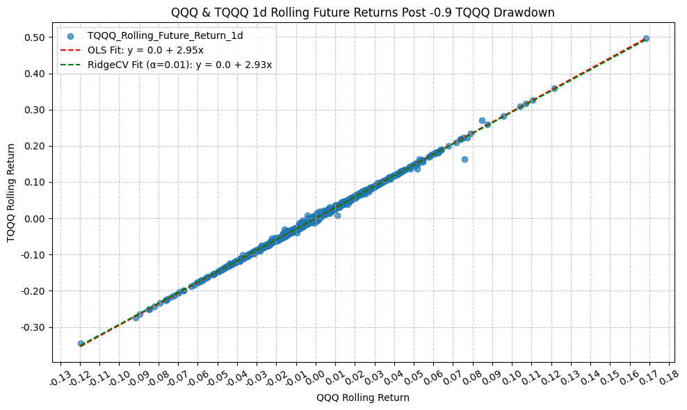
                                  OLS Regression Results
=========================================================================================
Dep. Variable:     TQQQ_Rolling_Future_Return_1d   R-squared:                       0.999
Model:                                       OLS   Adj. R-squared:                  0.999
Method:                            Least Squares   F-statistic:                 3.965e+06
Date:                           Mon, 23 Mar 2026   Prob (F-statistic):               0.00
Time:                                   22:01:50   Log-Likelihood:                 24386.
No. Observations:                           4909   AIC:                        -4.877e+04
Df Residuals:                               4907   BIC:                        -4.875e+04
Df Model:                                      1
Covariance Type:                       nonrobust
================================================================================================
                                   coef    std err          t      P>|t|      [0.025      0.975]
------------------------------------------------------------------------------------------------
const                         7.129e-06   2.41e-05      0.296      0.767      -4e-05    5.43e-05
QQQ_Rolling_Future_Return_1d     2.9508      0.001   1991.332      0.000       2.948       2.954
==============================================================================
Omnibus:                     7546.968   Durbin-Watson:                   2.588
Prob(Omnibus):                  0.000   Jarque-Bera (JB):         28785736.106
Skew:                          -8.740   Prob(JB):                         0.00
Kurtosis:                     377.736   Cond. No.                         61.6
==============================================================================

Notes:
[1] Standard Errors assume that the covariance matrix of the errors is correctly specified.
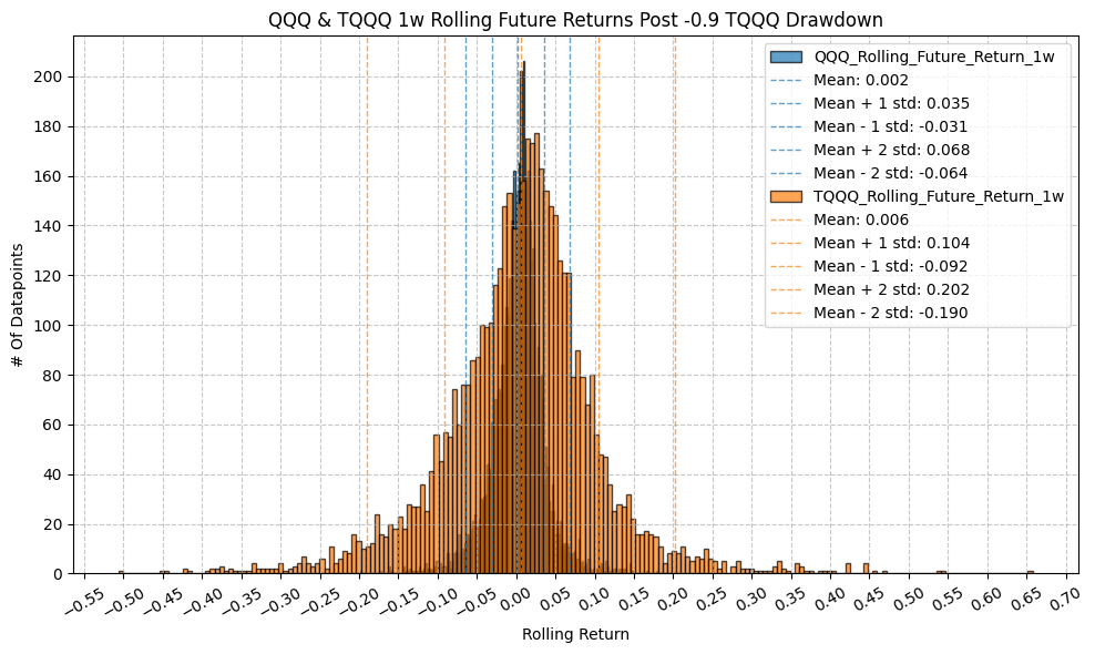
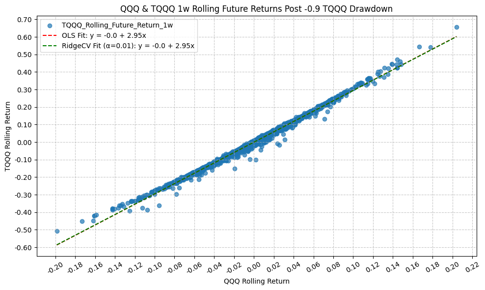
                                  OLS Regression Results
=========================================================================================
Dep. Variable:     TQQQ_Rolling_Future_Return_1w   R-squared:                       0.994
Model:                                       OLS   Adj. R-squared:                  0.994
Method:                            Least Squares   F-statistic:                 8.425e+05
Date:                           Mon, 23 Mar 2026   Prob (F-statistic):               0.00
Time:                                   22:01:52   Log-Likelihood:                 17077.
No. Observations:                           4909   AIC:                        -3.415e+04
Df Residuals:                               4907   BIC:                        -3.414e+04
Df Model:                                      1
Covariance Type:                       nonrobust
================================================================================================
                                   coef    std err          t      P>|t|      [0.025      0.975]
------------------------------------------------------------------------------------------------
const                           -0.0005      0.000     -4.398      0.000      -0.001      -0.000
QQQ_Rolling_Future_Return_1w     2.9537      0.003    917.898      0.000       2.947       2.960
==============================================================================
Omnibus:                     3458.331   Durbin-Watson:                   0.891
Prob(Omnibus):                  0.000   Jarque-Bera (JB):           430375.683
Skew:                          -2.502   Prob(JB):                         0.00
Kurtosis:                      48.597   Cond. No.                         30.2
==============================================================================

Notes:
[1] Standard Errors assume that the covariance matrix of the errors is correctly specified.
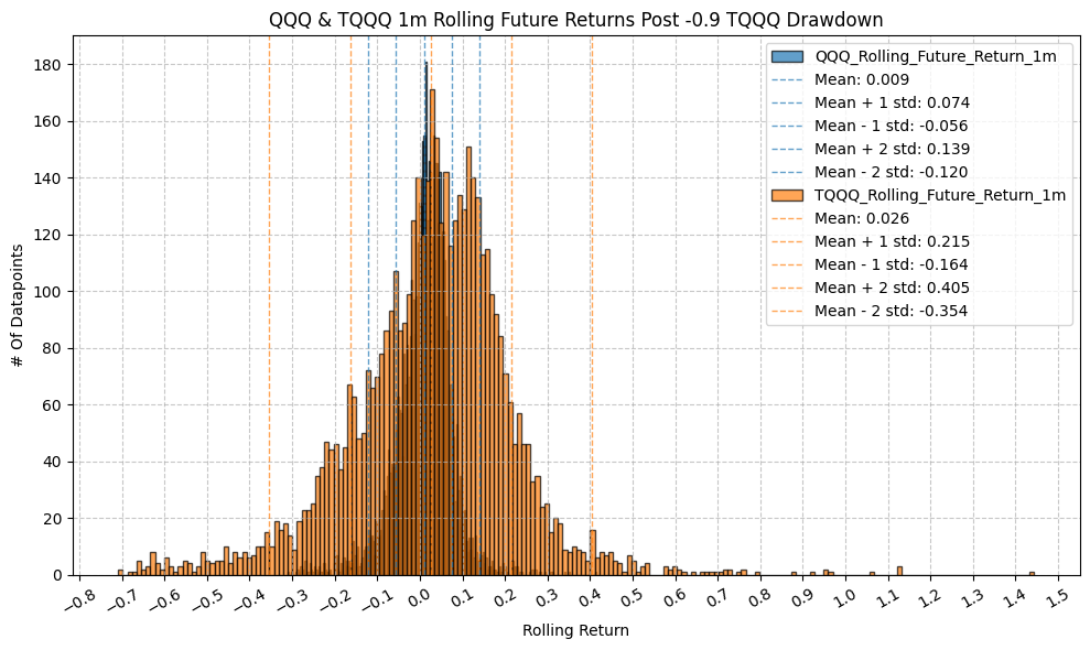
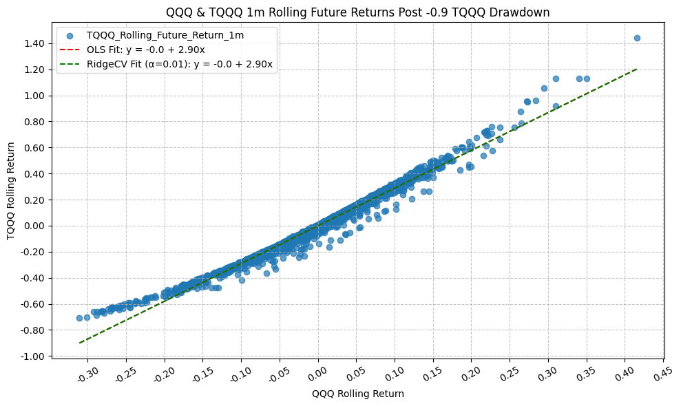
                                  OLS Regression Results
=========================================================================================
Dep. Variable:     TQQQ_Rolling_Future_Return_1m   R-squared:                       0.982
Model:                                       OLS   Adj. R-squared:                  0.982
Method:                            Least Squares   F-statistic:                 2.620e+05
Date:                           Mon, 23 Mar 2026   Prob (F-statistic):               0.00
Time:                                   22:01:53   Log-Likelihood:                 11004.
No. Observations:                           4909   AIC:                        -2.200e+04
Df Residuals:                               4907   BIC:                        -2.199e+04
Df Model:                                      1
Covariance Type:                       nonrobust
================================================================================================
                                   coef    std err          t      P>|t|      [0.025      0.975]
------------------------------------------------------------------------------------------------
const                           -0.0014      0.000     -3.884      0.000      -0.002      -0.001
QQQ_Rolling_Future_Return_1m     2.8966      0.006    511.823      0.000       2.886       2.908
==============================================================================
Omnibus:                     1234.759   Durbin-Watson:                   0.289
Prob(Omnibus):                  0.000   Jarque-Bera (JB):            81518.307
Skew:                           0.182   Prob(JB):                         0.00
Kurtosis:                      22.960   Cond. No.                         15.4
==============================================================================

Notes:
[1] Standard Errors assume that the covariance matrix of the errors is correctly specified.
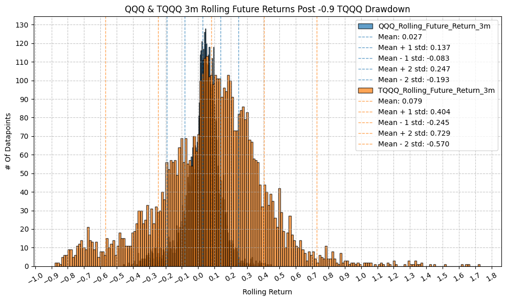

                                  OLS Regression Results
=========================================================================================
Dep. Variable:     TQQQ_Rolling_Future_Return_3m   R-squared:                       0.964
Model:                                       OLS   Adj. R-squared:                  0.964
Method:                            Least Squares   F-statistic:                 1.297e+05
Date:                           Mon, 23 Mar 2026   Prob (F-statistic):               0.00
Time:                                   22:01:55   Log-Likelihood:                 6687.8
No. Observations:                           4909   AIC:                        -1.337e+04
Df Residuals:                               4907   BIC:                        -1.336e+04
Df Model:                                      1
Covariance Type:                       nonrobust
================================================================================================
                                   coef    std err          t      P>|t|      [0.025      0.975]
------------------------------------------------------------------------------------------------
const                            0.0002      0.001      0.215      0.829      -0.002       0.002
QQQ_Rolling_Future_Return_3m     2.8959      0.008    360.175      0.000       2.880       2.912
==============================================================================
Omnibus:                     1438.612   Durbin-Watson:                   0.111
Prob(Omnibus):                  0.000   Jarque-Bera (JB):            18131.281
Skew:                           1.037   Prob(JB):                         0.00
Kurtosis:                      12.184   Cond. No.                         9.10
==============================================================================

Notes:
[1] Standard Errors assume that the covariance matrix of the errors is correctly specified.
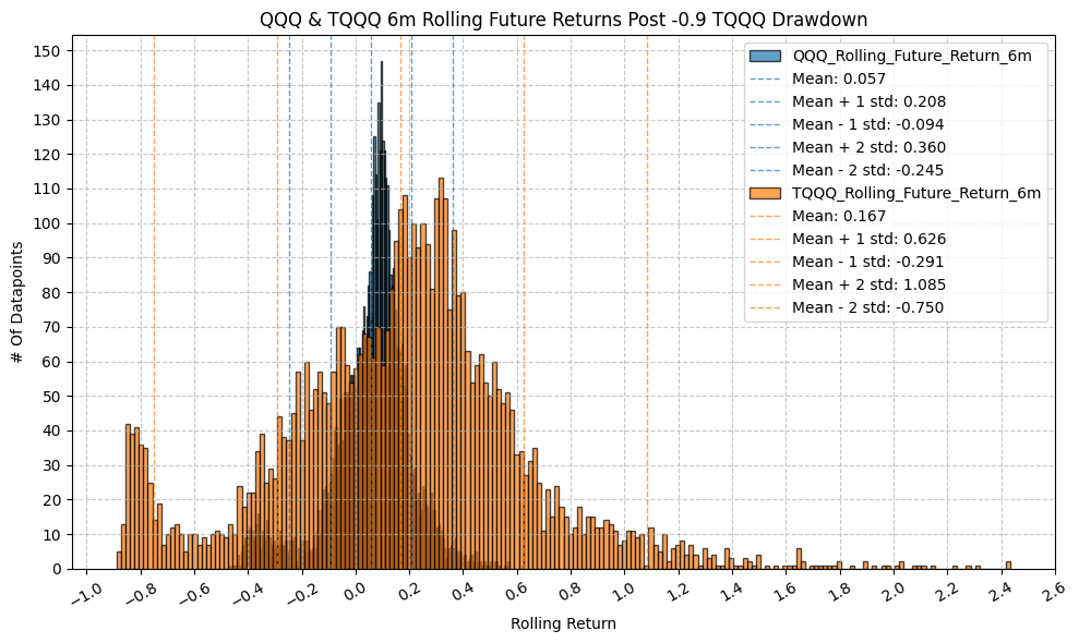
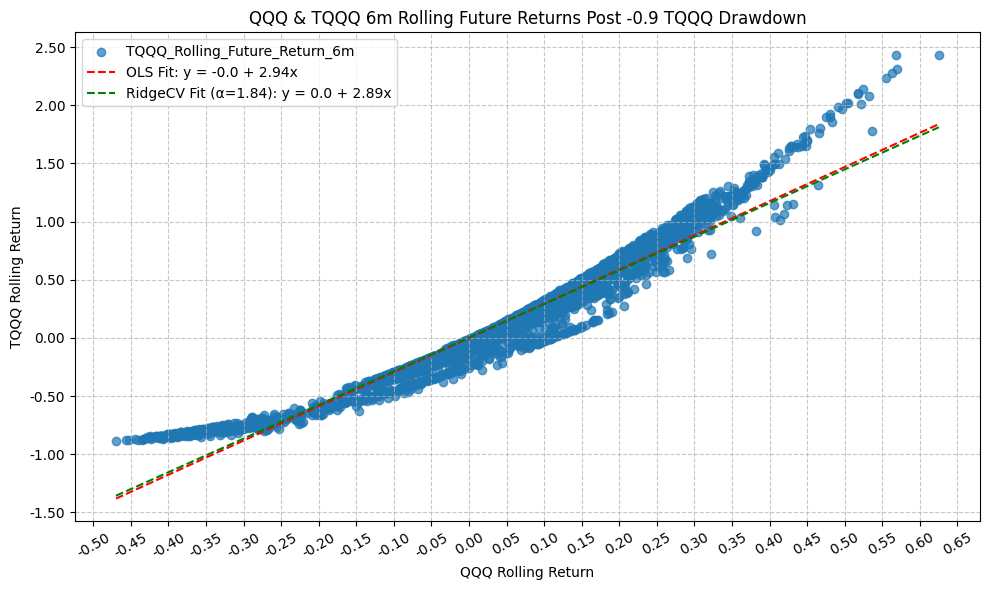
                                  OLS Regression Results
=========================================================================================
Dep. Variable:     TQQQ_Rolling_Future_Return_6m   R-squared:                       0.940
Model:                                       OLS   Adj. R-squared:                  0.940
Method:                            Least Squares   F-statistic:                 7.744e+04
Date:                           Mon, 23 Mar 2026   Prob (F-statistic):               0.00
Time:                                   22:01:56   Log-Likelihood:                 3783.0
No. Observations:                           4909   AIC:                            -7562.
Df Residuals:                               4907   BIC:                            -7549.
Df Model:                                      1
Covariance Type:                       nonrobust
================================================================================================
                                   coef    std err          t      P>|t|      [0.025      0.975]
------------------------------------------------------------------------------------------------
const                           -0.0006      0.002     -0.378      0.705      -0.004       0.003
QQQ_Rolling_Future_Return_6m     2.9398      0.011    278.286      0.000       2.919       2.960
==============================================================================
Omnibus:                     1092.173   Durbin-Watson:                   0.063
Prob(Omnibus):                  0.000   Jarque-Bera (JB):             5026.717
Skew:                           1.005   Prob(JB):                         0.00
Kurtosis:                       7.531   Cond. No.                         6.63
==============================================================================

Notes:
[1] Standard Errors assume that the covariance matrix of the errors is correctly specified.
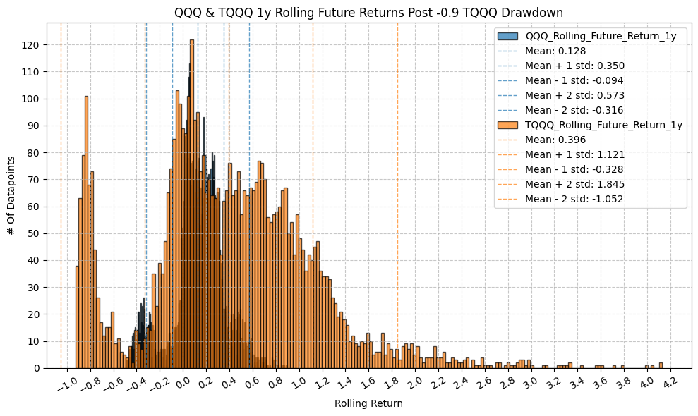
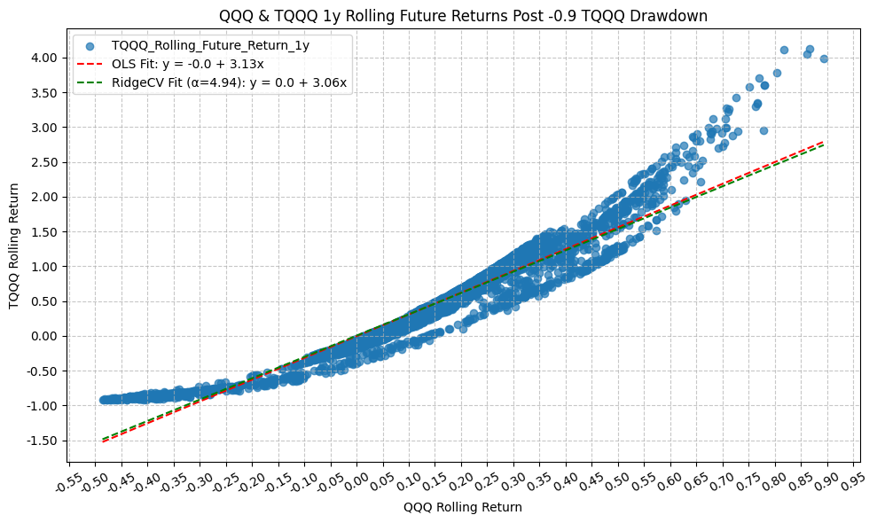
                                  OLS Regression Results
=========================================================================================
Dep. Variable:     TQQQ_Rolling_Future_Return_1y   R-squared:                       0.921
Model:                                       OLS   Adj. R-squared:                  0.921
Method:                            Least Squares   F-statistic:                 5.687e+04
Date:                           Mon, 23 Mar 2026   Prob (F-statistic):               0.00
Time:                                   22:01:58   Log-Likelihood:                 835.19
No. Observations:                           4909   AIC:                            -1666.
Df Residuals:                               4907   BIC:                            -1653.
Df Model:                                      1
Covariance Type:                       nonrobust
================================================================================================
                                   coef    std err          t      P>|t|      [0.025      0.975]
------------------------------------------------------------------------------------------------
const                           -0.0041      0.003     -1.223      0.222      -0.011       0.002
QQQ_Rolling_Future_Return_1y     3.1266      0.013    238.485      0.000       3.101       3.152
==============================================================================
Omnibus:                     1289.761   Durbin-Watson:                   0.048
Prob(Omnibus):                  0.000   Jarque-Bera (JB):             5901.804
Skew:                           1.201   Prob(JB):                         0.00
Kurtosis:                       7.804   Cond. No.                         4.58
==============================================================================

Notes:
[1] Standard Errors assume that the covariance matrix of the errors is correctly specified.
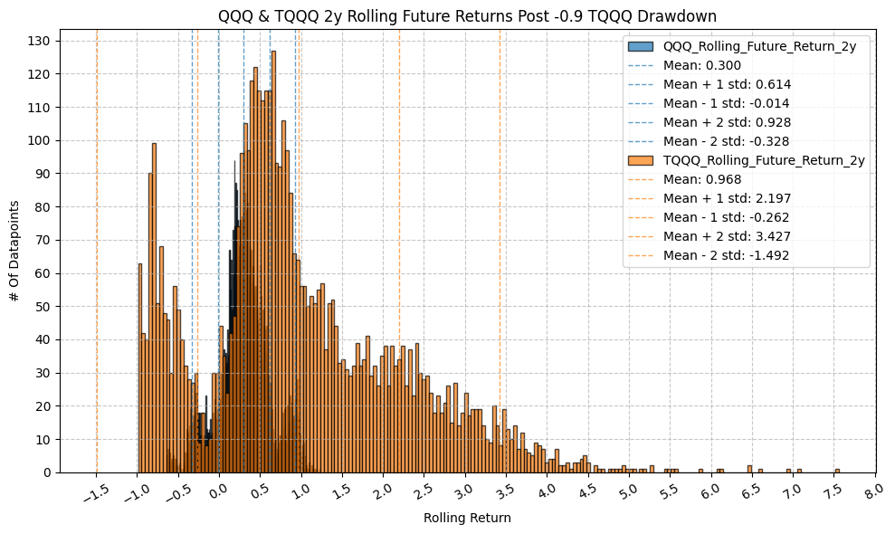
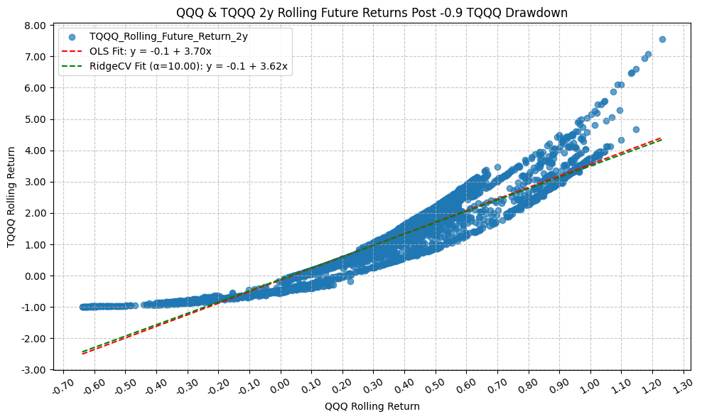
                                  OLS Regression Results
=========================================================================================
Dep. Variable:     TQQQ_Rolling_Future_Return_2y   R-squared:                       0.890
Model:                                       OLS   Adj. R-squared:                  0.890
Method:                            Least Squares   F-statistic:                 3.983e+04
Date:                           Mon, 23 Mar 2026   Prob (F-statistic):               0.00
Time:                                   22:02:00   Log-Likelihood:                -2555.1
No. Observations:                           4909   AIC:                             5114.
Df Residuals:                               4907   BIC:                             5127.
Df Model:                                      1
Covariance Type:                       nonrobust
================================================================================================
                                   coef    std err          t      P>|t|      [0.025      0.975]
------------------------------------------------------------------------------------------------
const                           -0.1417      0.008    -17.612      0.000      -0.157      -0.126
QQQ_Rolling_Future_Return_2y     3.6958      0.019    199.587      0.000       3.660       3.732
==============================================================================
Omnibus:                     1260.114   Durbin-Watson:                   0.024
Prob(Omnibus):                  0.000   Jarque-Bera (JB):             4504.068
Skew:                           1.255   Prob(JB):                         0.00
Kurtosis:                       6.965   Cond. No.                         3.50
==============================================================================

Notes:
[1] Standard Errors assume that the covariance matrix of the errors is correctly specified.

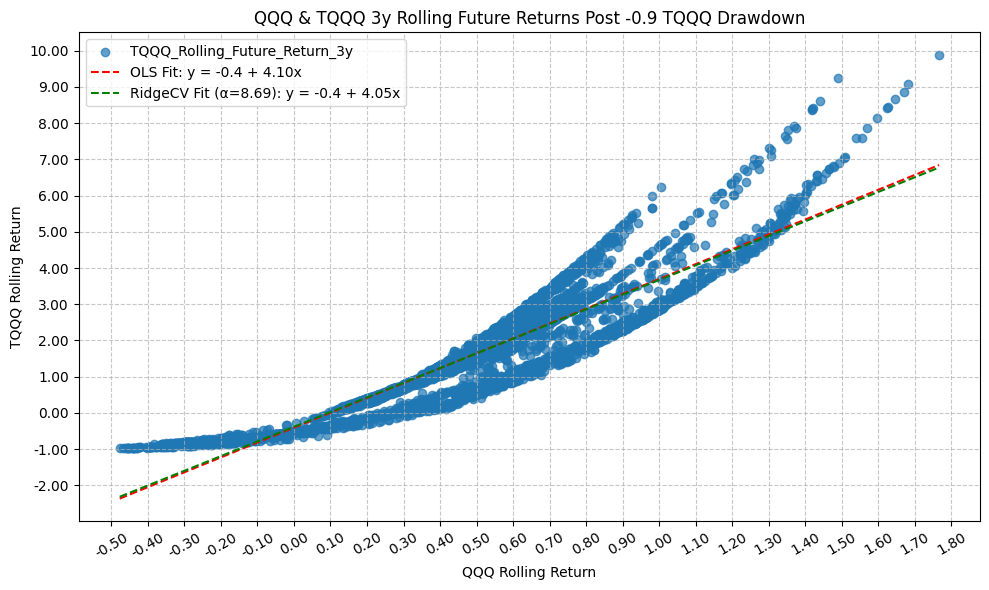
                                  OLS Regression Results
=========================================================================================
Dep. Variable:     TQQQ_Rolling_Future_Return_3y   R-squared:                       0.867
Model:                                       OLS   Adj. R-squared:                  0.867
Method:                            Least Squares   F-statistic:                 3.200e+04
Date:                           Mon, 23 Mar 2026   Prob (F-statistic):               0.00
Time:                                   22:02:02   Log-Likelihood:                -4386.9
No. Observations:                           4909   AIC:                             8778.
Df Residuals:                               4907   BIC:                             8791.
Df Model:                                      1
Covariance Type:                       nonrobust
================================================================================================
                                   coef    std err          t      P>|t|      [0.025      0.975]
------------------------------------------------------------------------------------------------
const                           -0.4053      0.014    -29.517      0.000      -0.432      -0.378
QQQ_Rolling_Future_Return_3y     4.1031      0.023    178.879      0.000       4.058       4.148
==============================================================================
Omnibus:                      498.122   Durbin-Watson:                   0.020
Prob(Omnibus):                  0.000   Jarque-Bera (JB):             1119.080
Skew:                           0.622   Prob(JB):                    9.88e-244
Kurtosis:                       4.981   Cond. No.                         3.40
==============================================================================

Notes:
[1] Standard Errors assume that the covariance matrix of the errors is correctly specified.
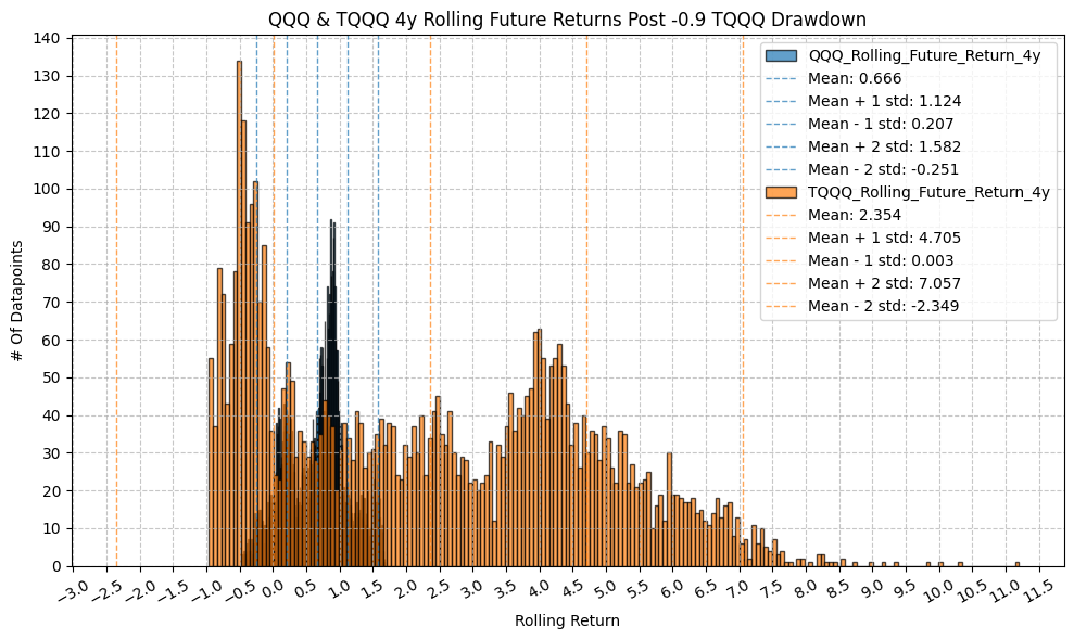
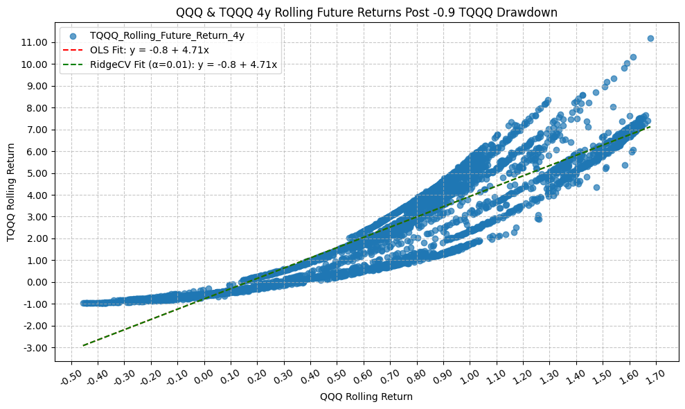
                                  OLS Regression Results
=========================================================================================
Dep. Variable:     TQQQ_Rolling_Future_Return_4y   R-squared:                       0.841
Model:                                       OLS   Adj. R-squared:                  0.841
Method:                            Least Squares   F-statistic:                 2.561e+04
Date:                           Mon, 23 Mar 2026   Prob (F-statistic):               0.00
Time:                                   22:02:03   Log-Likelihood:                -6578.4
No. Observations:                           4854   AIC:                         1.316e+04
Df Residuals:                               4852   BIC:                         1.317e+04
Df Model:                                      1
Covariance Type:                       nonrobust
================================================================================================
                                   coef    std err          t      P>|t|      [0.025      0.975]
------------------------------------------------------------------------------------------------
const                           -0.7780      0.024    -32.745      0.000      -0.825      -0.731
QQQ_Rolling_Future_Return_4y     4.7051      0.029    160.037      0.000       4.647       4.763
==============================================================================
Omnibus:                       37.797   Durbin-Watson:                   0.012
Prob(Omnibus):                  0.000   Jarque-Bera (JB):               38.924
Skew:                          -0.203   Prob(JB):                     3.53e-09
Kurtosis:                       3.167   Cond. No.                         3.31
==============================================================================

Notes:
[1] Standard Errors assume that the covariance matrix of the errors is correctly specified.
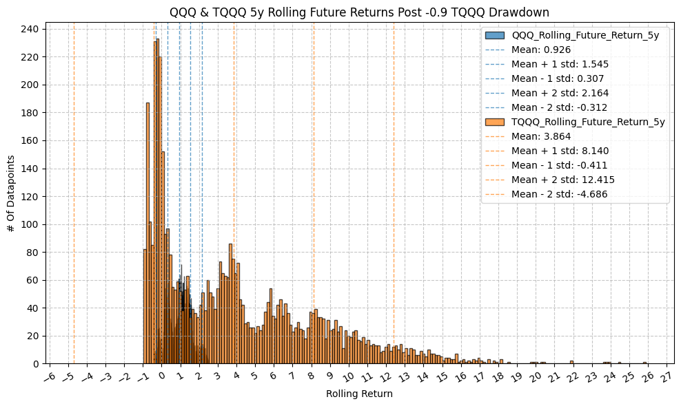
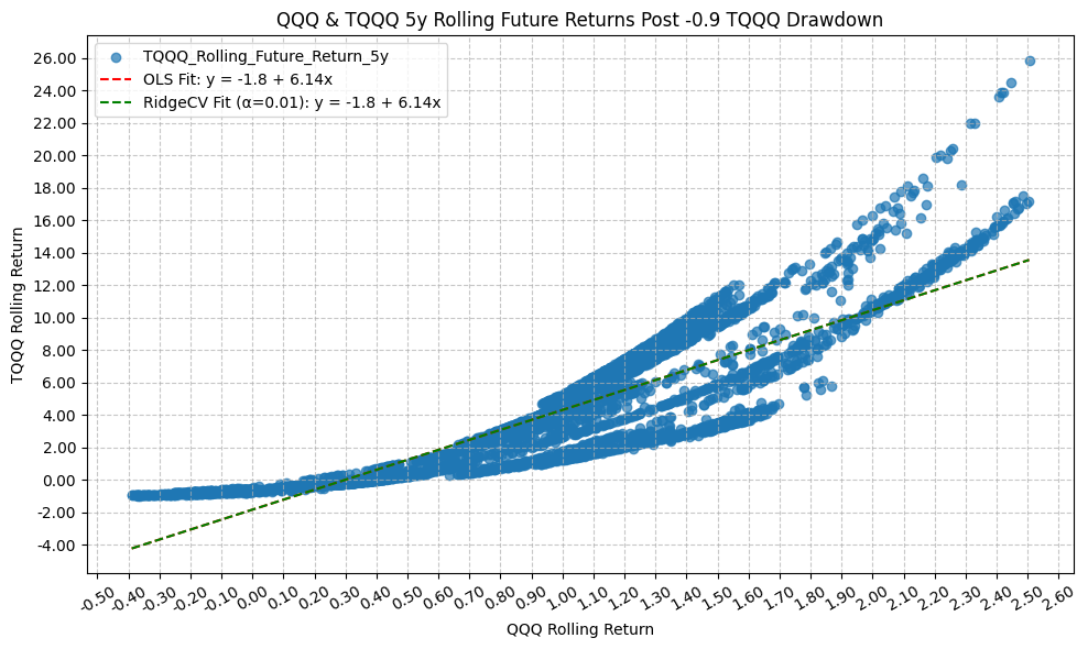
                                  OLS Regression Results
=========================================================================================
Dep. Variable:     TQQQ_Rolling_Future_Return_5y   R-squared:                       0.790
Model:                                       OLS   Adj. R-squared:                  0.790
Method:                            Least Squares   F-statistic:                 1.825e+04
Date:                           Mon, 23 Mar 2026   Prob (F-statistic):               0.00
Time:                                   22:02:05   Log-Likelihood:                -10152.
No. Observations:                           4854   AIC:                         2.031e+04
Df Residuals:                               4852   BIC:                         2.032e+04
Df Model:                                      1
Covariance Type:                       nonrobust
================================================================================================
                                   coef    std err          t      P>|t|      [0.025      0.975]
------------------------------------------------------------------------------------------------
const                           -1.8225      0.051    -35.999      0.000      -1.922      -1.723
QQQ_Rolling_Future_Return_5y     6.1390      0.045    135.095      0.000       6.050       6.228
==============================================================================
Omnibus:                      154.299   Durbin-Watson:                   0.011
Prob(Omnibus):                  0.000   Jarque-Bera (JB):              381.366
Skew:                           0.121   Prob(JB):                     1.54e-83
Kurtosis:                       4.352   Cond. No.                         3.32
==============================================================================

Notes:
[1] Standard Errors assume that the covariance matrix of the errors is correctly specified.
Rolling Returns Following Drawdowns Deviation (QQQ & TQQQ) #
rolling_returns_positive_future_returns = pd.DataFrame(index=rolling_windows.keys(), data=rolling_windows.values())
rolling_returns_positive_future_returns.reset_index(inplace=True)
rolling_returns_positive_future_returns.rename(columns={"index":"Period", 0:"Days"}, inplace=True)

for drawdown in drawdown_levels:
    temp = rolling_returns_drawdown_stats.loc[rolling_returns_drawdown_stats["Drawdown"] == drawdown]
    temp = temp[["Period", "Positive_Future_Percentage"]]
    temp.rename(columns={"Positive_Future_Percentage" : f"Positive_Future_Percentage_Post_{drawdown}_Drawdown"}, inplace=True)
    rolling_returns_positive_future_returns = pd.merge(rolling_returns_positive_future_returns, temp, left_on="Period", right_on="Period", how="outer")
    rolling_returns_positive_future_returns.sort_values(by="Days", ascending=True, inplace=True)

rolling_returns_positive_future_returns.drop(columns={"Days"}, inplace=True)
rolling_returns_positive_future_returns.reset_index(drop=True, inplace=True)
pandas_set_decimal_places(2)
display(rolling_returns_positive_future_returns.set_index("Period"))
| Positive_Future_Percentage_Post_-0.1_Drawdown | Positive_Future_Percentage_Post_-0.2_Drawdown | Positive_Future_Percentage_Post_-0.3_Drawdown | Positive_Future_Percentage_Post_-0.4_Drawdown | Positive_Future_Percentage_Post_-0.5_Drawdown | Positive_Future_Percentage_Post_-0.6_Drawdown | Positive_Future_Percentage_Post_-0.7_Drawdown | Positive_Future_Percentage_Post_-0.8_Drawdown | Positive_Future_Percentage_Post_-0.9_Drawdown | |
|---|---|---|---|---|---|---|---|---|---|
| Period | |||||||||
| 1d | 0.54 | 0.54 | 0.54 | 0.54 | 0.54 | 0.55 | 0.54 | 0.54 | 0.54 |
| 1w | 0.56 | 0.56 | 0.56 | 0.56 | 0.56 | 0.57 | 0.57 | 0.56 | 0.56 |
| 1m | 0.60 | 0.60 | 0.59 | 0.59 | 0.60 | 0.60 | 0.60 | 0.60 | 0.60 |
| 3m | 0.64 | 0.64 | 0.64 | 0.64 | 0.64 | 0.64 | 0.65 | 0.65 | 0.65 |
| 6m | 0.66 | 0.66 | 0.66 | 0.66 | 0.66 | 0.67 | 0.69 | 0.68 | 0.68 |
| 1y | 0.71 | 0.71 | 0.71 | 0.71 | 0.71 | 0.71 | 0.73 | 0.74 | 0.73 |
| 2y | 0.73 | 0.74 | 0.75 | 0.75 | 0.75 | 0.75 | 0.78 | 0.80 | 0.81 |
| 3y | 0.74 | 0.75 | 0.76 | 0.76 | 0.76 | 0.77 | 0.78 | 0.78 | 0.78 |
| 4y | 0.73 | 0.74 | 0.75 | 0.75 | 0.75 | 0.75 | 0.76 | 0.76 | 0.75 |
| 5y | 0.73 | 0.74 | 0.75 | 0.75 | 0.75 | 0.75 | 0.76 | 0.76 | 0.76 |
plot_scatter(
    df=rolling_returns_positive_future_returns,
    x_plot_column="Period",
    y_plot_columns=[col for col in rolling_returns_positive_future_returns.columns if col != "Period"],
    title="TQQQ Future Return by Time Period Post Drawdown",
    x_label="Rolling Return Time Period",
    x_format="String",
    x_format_decimal_places=0,
    x_tick_spacing=1,
    x_tick_rotation=0,
    y_label="Positive Future Return Percentage",
    y_format="Decimal",
    y_format_decimal_places=2,
    y_tick_spacing="Auto",
    y_tick_rotation=0,
    plot_OLS_regression_line=False,
    OLS_column=None,
    plot_Ridge_regression_line=False,
    Ridge_column=None,
    plot_RidgeCV_regression_line=False,
    RidgeCV_column=None,
    regression_constant=False,
    grid=True,
    legend=True,
    export_plot=False,
    plot_file_name=None,
)
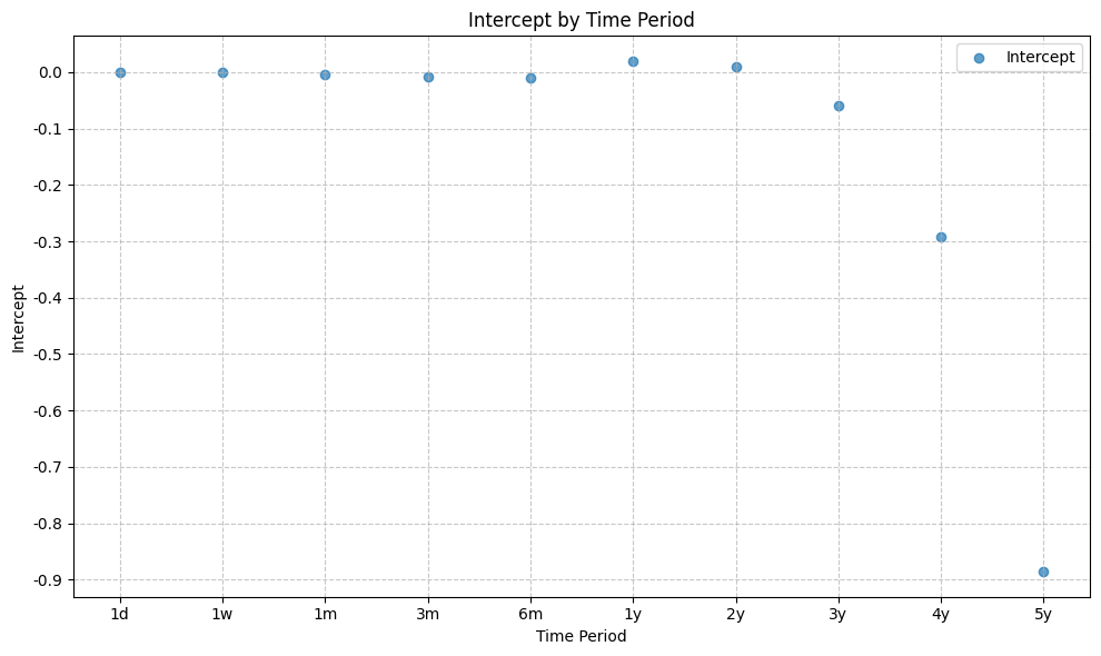
This plot summarizes the future rolling returns well. For rolling returns up to ~3 months following all drawdown levels, we see the rolling returns of TQQQ are positive ~65% of the time.
As we extend the time horizon, the percentage of positive rolling returns increases, which is consistent with the idea that the longer you hold through and post drawdown, the more likely you are to recover and achieve positive returns.
From a timing standpoint, this analysis suggests that the optimal time to buy TQQQ would be following a drawdown of 70% or more, and holding for at least 3 years. The data tells us that having a positive rolling return over time is ~75%.
One might consider the idea of allocating to TQQQ via a ladder, starting at a drawdown of 50%, and continuing to add to the position as the drawdown deepens, with the idea that the more severe the drawdown, the higher the expected future returns. However, this strategy could require enduring significant volatility, as one would be adding to the position during periods of paper losses.
SPY & UPRO #
Next, we will repeat the same analysis for SPY and UPRO, and see how the results compare to those of QQQ and TQQQ.
Acquire & Plot Data (SPY) #
First, let’s get the data for SPY. If we already have the desired data, we can load it from a local pickle file. Otherwise, we can download it from Yahoo Finance using the yf_pull_data function.
pandas_set_decimal_places(2)

yf_pull_data(
    base_directory=DATA_DIR,
    ticker="SPY",
    adjusted=False,
    source="Yahoo_Finance",
    asset_class="Exchange_Traded_Funds",
    excel_export=True,
    pickle_export=True,
    output_confirmation=False,
)

spy = load_data(
    base_directory=DATA_DIR,
    ticker="SPY",
    source="Yahoo_Finance",
    asset_class="Exchange_Traded_Funds",
    timeframe="Daily",
    file_format="pickle",
)

# Rename columns to "SPY_Close", etc.
spy = spy.rename(columns={
    "Adj Close": "SPY_Adj_Close",
    "Close": "SPY_Close",
    "High": "SPY_High",
    "Low": "SPY_Low",
    "Open": "SPY_Open",
    "Volume": "SPY_Volume"
})

display(spy)
| SPY_Adj_Close | SPY_Close | SPY_High | SPY_Low | SPY_Open | SPY_Volume | |
|---|---|---|---|---|---|---|
| Date | ||||||
| 1993-01-29 | 24.18 | 43.94 | 43.97 | 43.75 | 43.97 | 1003200 |
| 1993-02-01 | 24.35 | 44.25 | 44.25 | 43.97 | 43.97 | 480500 |
| 1993-02-02 | 24.40 | 44.34 | 44.38 | 44.12 | 44.22 | 201300 |
| 1993-02-03 | 24.66 | 44.81 | 44.84 | 44.38 | 44.41 | 529400 |
| 1993-02-04 | 24.76 | 45.00 | 45.09 | 44.47 | 44.97 | 531500 |
| ... | ... | ... | ... | ... | ... | ... |
| 2026-03-16 | 667.21 | 669.03 | 672.07 | 667.12 | 668.38 | 82023100 |
| 2026-03-17 | 668.96 | 670.79 | 674.44 | 669.70 | 672.39 | 87128000 |
| 2026-03-18 | 659.63 | 661.43 | 669.72 | 661.19 | 668.36 | 82062600 |
| 2026-03-19 | 658.00 | 659.80 | 662.98 | 655.17 | 656.97 | 111272500 |
| 2026-03-20 | 648.57 | 648.57 | 656.69 | 644.72 | 656.51 | 163617500 |
8342 rows × 6 columns
And the plot of the time series of partially adjusted close prices:
plot_time_series(
    df=spy,
    plot_start_date=None,
    plot_end_date=None,
    plot_columns=["SPY_Close"],
    title="SPY Close Price",
    x_label="Date",
    x_format="Year",
    x_tick_spacing=2,
    x_tick_rotation=30,
    y_label="Price ($)",
    y_format="Decimal",
    y_format_decimal_places=0,
    y_tick_spacing="Auto",
    y_tick_rotation=0,
    grid=True,
    legend=False,
    export_plot=False,
    plot_file_name=None,
)

Acquire & Plot Data (UPRO) #
Next, UPRO:
yf_pull_data(
    base_directory=DATA_DIR,
    ticker="UPRO",
    adjusted=False,
    source="Yahoo_Finance",
    asset_class="Exchange_Traded_Funds",
    excel_export=True,
    pickle_export=True,
    output_confirmation=False,
)

upro = load_data(
    base_directory=DATA_DIR,
    ticker="UPRO",
    source="Yahoo_Finance",
    asset_class="Exchange_Traded_Funds",
    timeframe="Daily",
    file_format="pickle",
)

# Rename columns to "UPRO_Close", etc.
upro = upro.rename(columns={
    "Adj Close": "UPRO_Adj_Close",
    "Close": "UPRO_Close",
    "High": "UPRO_High",
    "Low": "UPRO_Low",
    "Open": "UPRO_Open",
    "Volume": "UPRO_Volume"
})

display(upro)
| UPRO_Adj_Close | UPRO_Close | UPRO_High | UPRO_Low | UPRO_Open | UPRO_Volume | |
|---|---|---|---|---|---|---|
| Date | ||||||
| 2009-06-25 | 1.13 | 1.21 | 1.21 | 1.13 | 1.13 | 2577600 |
| 2009-06-26 | 1.13 | 1.20 | 1.21 | 1.18 | 1.20 | 13104000 |
| 2009-06-29 | 1.16 | 1.23 | 1.24 | 1.19 | 1.21 | 8690400 |
| 2009-06-30 | 1.13 | 1.20 | 1.24 | 1.18 | 1.23 | 17128800 |
| 2009-07-01 | 1.15 | 1.22 | 1.25 | 1.21 | 1.22 | 12038400 |
| ... | ... | ... | ... | ... | ... | ... |
| 2026-03-16 | 106.10 | 106.10 | 107.54 | 105.24 | 105.83 | 4607100 |
| 2026-03-17 | 106.92 | 106.92 | 108.67 | 106.60 | 107.70 | 2942600 |
| 2026-03-18 | 102.47 | 102.47 | 106.37 | 102.35 | 105.74 | 5114100 |
| 2026-03-19 | 101.63 | 101.63 | 103.11 | 99.48 | 100.27 | 5536600 |
| 2026-03-20 | 97.09 | 97.09 | 100.95 | 95.44 | 100.88 | 6060700 |
4210 rows × 6 columns
And the plot of the time series of partially adjusted close prices:
plot_time_series(
    df=upro,
    plot_start_date=None,
    plot_end_date=None,
    plot_columns=["UPRO_Close"],
    title="UPRO Close Price",
    x_label="Date",
    x_format="Year",
    x_tick_spacing=1,
    x_tick_rotation=30,
    y_label="Price ($)",
    y_format="Decimal",
    y_format_decimal_places=0,
    y_tick_spacing="Auto",
    y_tick_rotation=0,
    grid=True,
    legend=False,
    export_plot=False,
    plot_file_name=None,
)
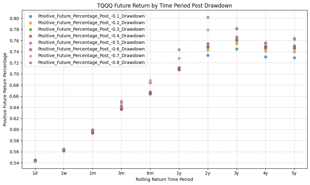
Looking at the close prices doesn’t give us a true picture of the magnitude of the difference in returns due to the leverage. In order to see that, we need to look at the cumulative returns and the drawdowns.
Calculate & Plot Cumulative Returns, Rolling Returns, and Drawdowns (SPY & UPRO) #
Next, we will calculate the cumulative returns, rolling returns, and drawdowns. This involves aligning the data to start with the inception of UPRO. For this excercise, we will not extrapolate the data for SPY back to 1993, but rather just align the data from the inception of UPRO in 2009.
etfs = ["SPY", "UPRO"]

# Merge dataframes and drop rows with missing values
spy_upro_aligned = upro.merge(spy, left_index=True, right_index=True, how='left')
spy_upro_aligned = spy_upro_aligned.dropna()

# Calculate cumulative returns
for etf in etfs:
    spy_upro_aligned[f"{etf}_Return"] = spy_upro_aligned[f"{etf}_Close"].pct_change()
    spy_upro_aligned[f"{etf}_Cumulative_Return"] = (1 + spy_upro_aligned[f"{etf}_Return"]).cumprod() - 1
    spy_upro_aligned[f"{etf}_Cumulative_Return_Plus_One"] = 1 + spy_upro_aligned[f"{etf}_Cumulative_Return"]
    spy_upro_aligned[f"{etf}_Rolling_Max"] = spy_upro_aligned[f"{etf}_Cumulative_Return_Plus_One"].cummax()
    spy_upro_aligned[f"{etf}_Drawdown"] = spy_upro_aligned[f"{etf}_Cumulative_Return_Plus_One"] / spy_upro_aligned[f"{etf}_Rolling_Max"] - 1
    spy_upro_aligned.drop(columns=[f"{etf}_Cumulative_Return_Plus_One", f"{etf}_Rolling_Max"], inplace=True)

# Define rolling windows in trading days
rolling_windows = {
    '1d': 1,      # 1 day
    '1w': 5,      # 1 week (5 trading days)
    '1m': 21,     # 1 month (~21 trading days)
    '3m': 63,     # 3 months (~63 trading days)
    '6m': 126,    # 6 months (~126 trading days)
    '1y': 252,    # 1 year (~252 trading days)
    '2y': 504,    # 2 years (~504 trading days)
    '3y': 756,    # 3 years (~756 trading days)
    '4y': 1008,   # 4 years (~1008 trading days)
    '5y': 1260,   # 5 years (~1260 trading days)
}

# Calculate rolling returns for each ETF and each window
for etf in etfs:
    for period_name, window in rolling_windows.items():
        spy_upro_aligned[f"{etf}_Rolling_Return_{period_name}"] = (
            spy_upro_aligned[f"{etf}_Close"].pct_change(periods=window)
        )

display(spy_upro_aligned)
| UPRO_Adj_Close | UPRO_Close | UPRO_High | UPRO_Low | UPRO_Open | UPRO_Volume | SPY_Adj_Close | SPY_Close | SPY_High | SPY_Low | ... | UPRO_Rolling_Return_1d | UPRO_Rolling_Return_1w | UPRO_Rolling_Return_1m | UPRO_Rolling_Return_3m | UPRO_Rolling_Return_6m | UPRO_Rolling_Return_1y | UPRO_Rolling_Return_2y | UPRO_Rolling_Return_3y | UPRO_Rolling_Return_4y | UPRO_Rolling_Return_5y | |
|---|---|---|---|---|---|---|---|---|---|---|---|---|---|---|---|---|---|---|---|---|---|
| Date | |||||||||||||||||||||
| 2009-06-25 | 1.13 | 1.21 | 1.21 | 1.13 | 1.13 | 2577600 | 68.20 | 92.08 | 92.17 | 89.57 | ... | NaN | NaN | NaN | NaN | NaN | NaN | NaN | NaN | NaN | NaN |
| 2009-06-26 | 1.13 | 1.20 | 1.21 | 1.18 | 1.20 | 13104000 | 68.03 | 91.84 | 92.24 | 91.27 | ... | -0.01 | NaN | NaN | NaN | NaN | NaN | NaN | NaN | NaN | NaN |
| 2009-06-29 | 1.16 | 1.23 | 1.24 | 1.19 | 1.21 | 8690400 | 68.66 | 92.70 | 92.82 | 91.60 | ... | 0.03 | NaN | NaN | NaN | NaN | NaN | NaN | NaN | NaN | NaN |
| 2009-06-30 | 1.13 | 1.20 | 1.24 | 1.18 | 1.23 | 17128800 | 68.11 | 91.95 | 93.06 | 91.27 | ... | -0.02 | NaN | NaN | NaN | NaN | NaN | NaN | NaN | NaN | NaN |
| 2009-07-01 | 1.15 | 1.22 | 1.25 | 1.21 | 1.22 | 12038400 | 68.39 | 92.33 | 93.23 | 92.21 | ... | 0.01 | NaN | NaN | NaN | NaN | NaN | NaN | NaN | NaN | NaN |
| ... | ... | ... | ... | ... | ... | ... | ... | ... | ... | ... | ... | ... | ... | ... | ... | ... | ... | ... | ... | ... | ... |
| 2026-03-16 | 106.10 | 106.10 | 107.54 | 105.24 | 105.83 | 4607100 | 667.21 | 669.03 | 672.07 | 667.12 | ... | 0.03 | -0.04 | -0.07 | -0.11 | -0.01 | 0.49 | 0.61 | 2.13 | 1.13 | 1.53 |
| 2026-03-17 | 106.92 | 106.92 | 108.67 | 106.60 | 107.70 | 2942600 | 668.96 | 670.79 | 674.44 | 669.70 | ... | 0.01 | -0.03 | -0.06 | -0.08 | -0.02 | 0.42 | 0.57 | 2.30 | 0.98 | 1.51 |
| 2026-03-18 | 102.47 | 102.47 | 106.37 | 102.35 | 105.74 | 5114100 | 659.63 | 661.43 | 669.72 | 661.19 | ... | -0.04 | -0.07 | -0.10 | -0.11 | -0.05 | 0.33 | 0.51 | 2.18 | 0.93 | 1.33 |
| 2026-03-19 | 101.63 | 101.63 | 103.11 | 99.48 | 100.27 | 5536600 | 658.00 | 659.80 | 662.98 | 655.17 | ... | -0.01 | -0.03 | -0.12 | -0.11 | -0.06 | 0.36 | 0.51 | 2.00 | 0.99 | 1.30 |
| 2026-03-20 | 97.09 | 97.09 | 100.95 | 95.44 | 100.88 | 6060700 | 648.57 | 648.57 | 656.69 | 644.72 | ... | -0.04 | -0.06 | -0.15 | -0.12 | -0.11 | 0.26 | 0.48 | 1.92 | 0.94 | 1.16 |
4210 rows × 38 columns
And now the plot for the cumulative returns:
plot_time_series(
    df=spy_upro_aligned,
    plot_start_date=None,
    plot_end_date=None,
    plot_columns=["SPY_Cumulative_Return", "UPRO_Cumulative_Return"],
    title="Cumulative Returns",
    x_label="Date",
    x_format="Year",
    x_tick_spacing=1,
    x_tick_rotation=30,
    y_label="Cumulative Return",
    y_format="Decimal",
    y_format_decimal_places=0,
    y_tick_spacing="Auto",
    y_tick_rotation=0,
    grid=True,
    legend=True,
    export_plot=False,
    plot_file_name=None,
)
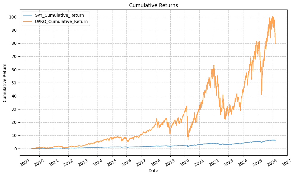
And the drawdown plot:
plot_time_series(
    df=spy_upro_aligned,
    plot_start_date=None,
    plot_end_date=None,
    plot_columns=["SPY_Drawdown", "UPRO_Drawdown"],
    title="Drawdowns",
    x_label="Date",
    x_format="Year",
    x_tick_spacing=1,
    x_tick_rotation=30,
    y_label="Drawdown",
    y_format="Percentage",
    y_format_decimal_places=0,
    y_tick_spacing="Auto",
    y_tick_rotation=0,
    grid=True,
    legend=True,
    export_plot=False,
    plot_file_name=None,
)

Summary Statistics (SPY & UPRO) #
Looking at the summary statistics further confirms our intuitions about the volatility and drawdowns.
spy_sum_stats = summary_stats(
    fund_list=["SPY"],
    df=spy_upro_aligned[["SPY_Return"]],
    period="Daily",
    use_calendar_days=False,
    excel_export=False,
    pickle_export=False,
    output_confirmation=False,
)

upro_sum_stats = summary_stats(
    fund_list=["UPRO"],
    df=spy_upro_aligned[["UPRO_Return"]],
    period="Daily",
    use_calendar_days=False,
    excel_export=False,
    pickle_export=False,
    output_confirmation=False,
)

sum_stats = pd.concat([spy_sum_stats, upro_sum_stats])

display(sum_stats)
| Annual Mean Return (Arithmetic) | Annualized Volatility | Annualized Sharpe Ratio | CAGR (Geometric) | Daily Max Return | Daily Max Return (Date) | Daily Min Return | Daily Min Return (Date) | Max Drawdown | Peak | Trough | Recovery Date | Calendar Days to Recovery | MAR Ratio | |
|---|---|---|---|---|---|---|---|---|---|---|---|---|---|---|
| SPY_Return | 0.13 | 0.17 | 0.77 | 0.12 | 0.11 | 2025-04-09 | -0.11 | 2020-03-16 | -0.34 | 2020-02-19 | 2020-03-23 | 2020-08-18 | 148 | 0.36 |
| UPRO_Return | 0.40 | 0.51 | 0.77 | 0.30 | 0.28 | 2020-03-24 | -0.35 | 2020-03-16 | -0.77 | 2020-02-19 | 2020-03-23 | 2021-01-08 | 291 | 0.39 |
Plot Returns & Verify Beta (SPY & UPRO) #
Before we look at the rolling returns, let us first verify that the daily returns for UPRO are in fact ~3x those of SPY.
plot_scatter(
    df=spy_upro_aligned,
    x_plot_column="SPY_Return",
    y_plot_columns=["UPRO_Return"],
    title="SPY & UPRO Returns",
    x_label="SPY Return",
    x_format="Decimal",
    x_format_decimal_places=2,
    x_tick_spacing="Auto",
    x_tick_rotation=30,
    y_label="UPRO Return",
    y_format="Decimal",
    y_format_decimal_places=2,
    y_tick_spacing="Auto",
    y_tick_rotation=0,
    plot_OLS_regression_line=True,
    OLS_column="UPRO_Return",
    plot_Ridge_regression_line=False,
    Ridge_column=None,
    plot_RidgeCV_regression_line=True,
    RidgeCV_column="UPRO_Return",
    regression_constant=True,
    grid=True,
    legend=True,
    export_plot=False,
    plot_file_name=None,
)
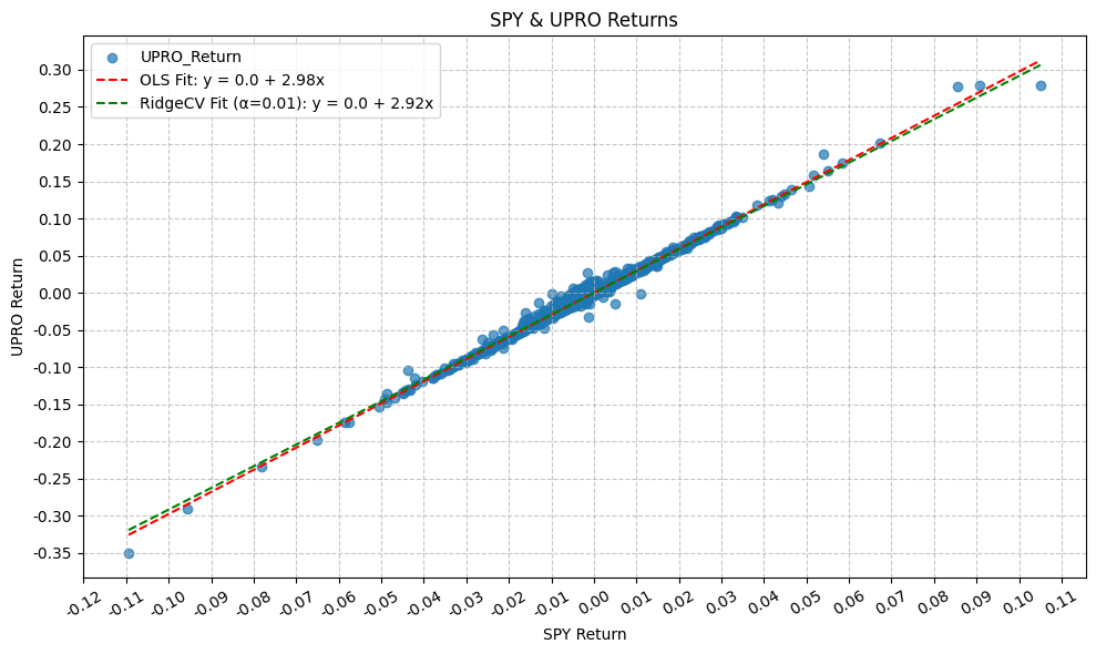
model = run_linear_regression(
    df=spy_upro_aligned,
    x_plot_column="SPY_Return",
    y_plot_column="UPRO_Return",
    regression_model="OLS-statsmodels",
    regression_constant=True,
)

print(model.summary())
                            OLS Regression Results
==============================================================================
Dep. Variable:            UPRO_Return   R-squared:                       0.994
Model:                            OLS   Adj. R-squared:                  0.994
Method:                 Least Squares   F-statistic:                 6.751e+05
Date:                Mon, 23 Mar 2026   Prob (F-statistic):               0.00
Time:                        22:02:16   Log-Likelihood:                 19172.
No. Observations:                4209   AIC:                        -3.834e+04
Df Residuals:                    4207   BIC:                        -3.833e+04
Df Model:                           1
Covariance Type:            nonrobust
==============================================================================
                 coef    std err          t      P>|t|      [0.025      0.975]
------------------------------------------------------------------------------
const        1.83e-05   3.93e-05      0.466      0.641   -5.87e-05    9.53e-05
SPY_Return     2.9758      0.004    821.652      0.000       2.969       2.983
==============================================================================
Omnibus:                     2682.534   Durbin-Watson:                   2.589
Prob(Omnibus):                  0.000   Jarque-Bera (JB):           515898.895
Skew:                           1.985   Prob(JB):                         0.00
Kurtosis:                      57.092   Cond. No.                         92.3
==============================================================================

Notes:
[1] Standard Errors assume that the covariance matrix of the errors is correctly specified.
Similar to QQQ/TQQQ, this plot makes sense and we can see that there is a strong clustering of points, but we double check with the regression, regressing the UPRO daily return (y) on the SPY daily return (X).
Extrapolate Data (SPY & UPRO) #
We will now extrapolate the returns of SPY to backfill the data from the inception of SPY in 1993 to the inception of UPRO in 2009. For this, we’ll use the coefficient of 2.98 that we found in the regression results above.
# Set leverage multiplier based on regression coefficient
LEVERAGE_MULTIPLIER = model.params[1]

# Merge dataframes and extrapolate return values for SPY back to 1993 using the leverage multiplier
spy_upro_extrap = spy[["SPY_Close"]].merge(upro[["UPRO_Close"]], left_index=True, right_index=True, how='left')

etfs = ["SPY", "UPRO"]

# Calculate cumulative returns
for etf in etfs:
    spy_upro_extrap[f"{etf}_Return"] = spy_upro_extrap[f"{etf}_Close"].pct_change()

# Extrapolate UPRO returns for missing values
spy_upro_extrap["UPRO_Return"] = spy_upro_extrap["UPRO_Return"].fillna(LEVERAGE_MULTIPLIER * spy_upro_extrap["SPY_Return"])

# Find the first valid UPRO_Close index and value
first_valid_idx = spy_upro_extrap['UPRO_Close'].first_valid_index()
print(first_valid_idx)
first_valid_price = spy_upro_extrap.loc[first_valid_idx, 'UPRO_Close']
print(first_valid_price)
2009-06-25 00:00:00
1.205556035041809
Before we extrapolate, let’s first look at the data we have for SPY and UPRO around the inception of UPRO in 2009:
# Check values around the first valid index
pandas_set_decimal_places(4)
display(spy_upro_extrap.loc["2009-06-20":"2009-06-30"])
| SPY_Close | UPRO_Close | SPY_Return | UPRO_Return | |
|---|---|---|---|---|
| Date | ||||
| 2009-06-22 | 89.2800 | NaN | -0.0300 | -0.0892 |
| 2009-06-23 | 89.3500 | NaN | 0.0008 | 0.0023 |
| 2009-06-24 | 90.1200 | NaN | 0.0086 | 0.0256 |
| 2009-06-25 | 92.0800 | 1.2056 | 0.0217 | 0.0647 |
| 2009-06-26 | 91.8400 | 1.1993 | -0.0026 | -0.0052 |
| 2009-06-29 | 92.7000 | 1.2333 | 0.0094 | 0.0284 |
| 2009-06-30 | 91.9500 | 1.2039 | -0.0081 | -0.0239 |
Now, backfill the data for the UPRO close price:
# Iterate through the dataframe backwards
for i in range(spy_upro_extrap.index.get_loc(first_valid_idx) - 1, -1, -1):

    # The return that led to the price the next day
    current_return = spy_upro_extrap.iloc[i + 1]['UPRO_Return']

    # Get the next day's price
    next_price = spy_upro_extrap.iloc[i + 1]['UPRO_Close']

    # Price_{t} = Price_{t+1} / (1 + Return_{t})
    spy_upro_extrap.loc[spy_upro_extrap.index[i], 'UPRO_Close'] = next_price / (1 + current_return)
Finally, confirm the values are correct:
# Confirm values around the first valid index after extrapolation
display(spy_upro_extrap.loc["2009-06-20":"2009-06-30"])
| SPY_Close | UPRO_Close | SPY_Return | UPRO_Return | |
|---|---|---|---|---|
| Date | ||||
| 2009-06-22 | 89.2800 | 1.1014 | -0.0300 | -0.0892 |
| 2009-06-23 | 89.3500 | 1.1040 | 0.0008 | 0.0023 |
| 2009-06-24 | 90.1200 | 1.1323 | 0.0086 | 0.0256 |
| 2009-06-25 | 92.0800 | 1.2056 | 0.0217 | 0.0647 |
| 2009-06-26 | 91.8400 | 1.1993 | -0.0026 | -0.0052 |
| 2009-06-29 | 92.7000 | 1.2333 | 0.0094 | 0.0284 |
| 2009-06-30 | 91.9500 | 1.2039 | -0.0081 | -0.0239 |
And the complete DataFrame with the extrapolated values:
pandas_set_decimal_places(2)
display(spy_upro_extrap)
| SPY_Close | UPRO_Close | SPY_Return | UPRO_Return | |
|---|---|---|---|---|
| Date | ||||
| 1993-01-29 | 43.94 | 0.93 | NaN | NaN |
| 1993-02-01 | 44.25 | 0.95 | 0.01 | 0.02 |
| 1993-02-02 | 44.34 | 0.95 | 0.00 | 0.01 |
| 1993-02-03 | 44.81 | 0.98 | 0.01 | 0.03 |
| 1993-02-04 | 45.00 | 0.99 | 0.00 | 0.01 |
| ... | ... | ... | ... | ... |
| 2026-03-16 | 669.03 | 106.10 | 0.01 | 0.03 |
| 2026-03-17 | 670.79 | 106.92 | 0.00 | 0.01 |
| 2026-03-18 | 661.43 | 102.47 | -0.01 | -0.04 |
| 2026-03-19 | 659.80 | 101.63 | -0.00 | -0.01 |
| 2026-03-20 | 648.57 | 97.09 | -0.02 | -0.04 |
8342 rows × 4 columns
After the extrapolation, we now have the following plots for the prices, cumulative returns, and drawdowns:
etfs = ["SPY", "UPRO"]

# Calculate cumulative returns
for etf in etfs:
    spy_upro_extrap[f"{etf}_Return"] = spy_upro_extrap[f"{etf}_Close"].pct_change()
    spy_upro_extrap[f"{etf}_Cumulative_Return"] = (1 + spy_upro_extrap[f"{etf}_Return"]).cumprod() - 1
    spy_upro_extrap[f"{etf}_Cumulative_Return_Plus_One"] = 1 + spy_upro_extrap[f"{etf}_Cumulative_Return"]
    spy_upro_extrap[f"{etf}_Rolling_Max"] = spy_upro_extrap[f"{etf}_Cumulative_Return_Plus_One"].cummax()
    spy_upro_extrap[f"{etf}_Drawdown"] = spy_upro_extrap[f"{etf}_Cumulative_Return_Plus_One"] / spy_upro_extrap[f"{etf}_Rolling_Max"] - 1
    spy_upro_extrap.drop(columns=[f"{etf}_Cumulative_Return_Plus_One", f"{etf}_Rolling_Max"], inplace=True)
plot_time_series(
    df=spy_upro_extrap,
    plot_start_date=None,
    plot_end_date=None,
    plot_columns=["SPY_Close"],
    title="SPY Close Price",
    x_label="Date",
    x_format="Year",
    x_tick_spacing=2,
    x_tick_rotation=30,
    y_label="Price ($)",
    y_format="Decimal",
    y_format_decimal_places=0,
    y_tick_spacing="Auto",
    y_tick_rotation=0,
    grid=True,
    legend=False,
    export_plot=False,
    plot_file_name=None,
)

plot_time_series(
    df=spy_upro_extrap,
    plot_start_date=None,
    plot_end_date=None,
    plot_columns=["UPRO_Close"],
    title="UPRO Close Price",
    x_label="Date",
    x_format="Year",
    x_tick_spacing=2,
    x_tick_rotation=30,
    y_label="Price ($)",
    y_format="Decimal",
    y_format_decimal_places=0,
    y_tick_spacing="Auto",
    y_tick_rotation=0,
    grid=True,
    legend=False,
    export_plot=False,
    plot_file_name=None,
)
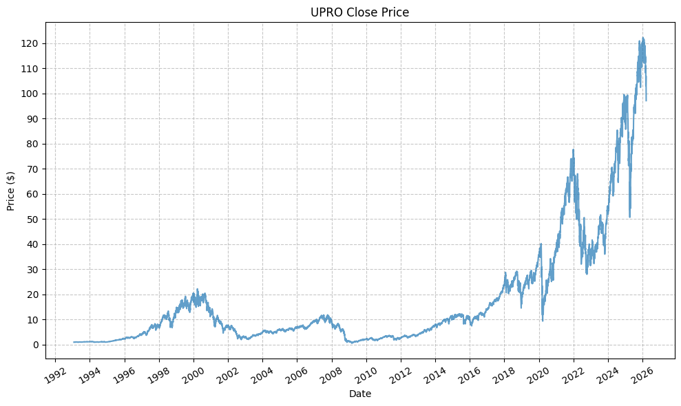
plot_time_series(
    df=spy_upro_extrap,
    plot_start_date=None,
    plot_end_date=None,
    plot_columns=["SPY_Cumulative_Return", "UPRO_Cumulative_Return"],
    title="Cumulative Returns",
    x_label="Date",
    x_format="Year",
    x_tick_spacing=2,
    x_tick_rotation=30,
    y_label="Cumulative Return",
    y_format="Decimal",
    y_format_decimal_places=0,
    y_tick_spacing="Auto",
    y_tick_rotation=0,
    grid=True,
    legend=True,
    export_plot=False,
    plot_file_name=None,
)
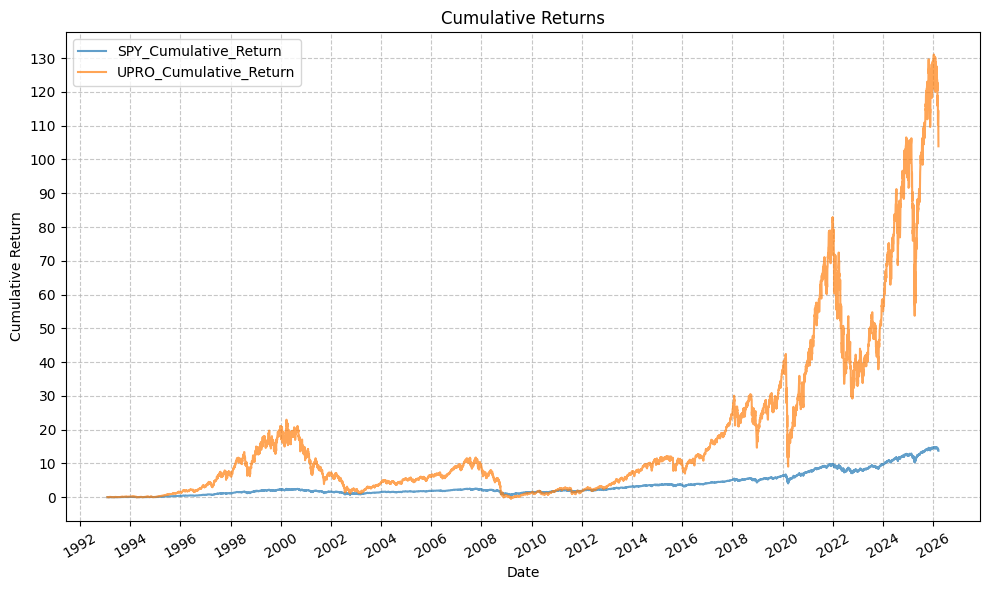
plot_time_series(
    df=spy_upro_extrap,
    plot_start_date=None,
    plot_end_date=None,
    plot_columns=["SPY_Drawdown", "UPRO_Drawdown"],
    title="Drawdowns",
    x_label="Date",
    x_format="Year",
    x_tick_spacing=1,
    x_tick_rotation=30,
    y_label="Drawdown",
    y_format="Percentage",
    y_format_decimal_places=0,
    y_tick_spacing="Auto",
    y_tick_rotation=0,
    grid=True,
    legend=True,
    export_plot=False,
    plot_file_name=None,
)
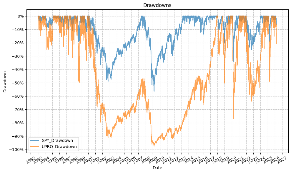
spy_extrap_sum_stats = summary_stats(
    fund_list=["SPY"],
    df=spy_upro_extrap[["SPY_Return"]],
    period="Daily",
    use_calendar_days=False,
    excel_export=False,
    pickle_export=False,
    output_confirmation=False,
)

upro_extrap_sum_stats = summary_stats(
    fund_list=["UPRO"],
    df=spy_upro_extrap[["UPRO_Return"]],
    period="Daily",
    use_calendar_days=False,
    excel_export=False,
    pickle_export=False,
    output_confirmation=False,
)

sum_stats = pd.concat([spy_sum_stats, upro_sum_stats, spy_extrap_sum_stats, upro_extrap_sum_stats])
sum_stats.index = ["SPY (2009 - Present)", "UPRO (2009 - Present)", "SPY (1993 - Present)", "UPRO Extrapolated (1993 - Present)"]

display(sum_stats)
| Annual Mean Return (Arithmetic) | Annualized Volatility | Annualized Sharpe Ratio | CAGR (Geometric) | Daily Max Return | Daily Max Return (Date) | Daily Min Return | Daily Min Return (Date) | Max Drawdown | Peak | Trough | Recovery Date | Calendar Days to Recovery | MAR Ratio | |
|---|---|---|---|---|---|---|---|---|---|---|---|---|---|---|
| SPY (2009 - Present) | 0.13 | 0.17 | 0.77 | 0.12 | 0.11 | 2025-04-09 | -0.11 | 2020-03-16 | -0.34 | 2020-02-19 | 2020-03-23 | 2020-08-18 | 148 | 0.36 |
| UPRO (2009 - Present) | 0.40 | 0.51 | 0.77 | 0.30 | 0.28 | 2020-03-24 | -0.35 | 2020-03-16 | -0.77 | 2020-02-19 | 2020-03-23 | 2021-01-08 | 291 | 0.39 |
| SPY (1993 - Present) | 0.10 | 0.19 | 0.53 | 0.08 | 0.15 | 2008-10-13 | -0.11 | 2020-03-16 | -0.56 | 2007-10-09 | 2009-03-09 | 2013-03-14 | 1466 | 0.15 |
| UPRO Extrapolated (1993 - Present) | 0.30 | 0.56 | 0.53 | 0.15 | 0.43 | 2008-10-13 | -0.35 | 2020-03-16 | -0.98 | 2000-03-24 | 2009-03-09 | 2017-11-30 | 3188 | 0.15 |
Interestingly, the maximum drawdown for UPRO is not as severe as that of TQQQ, which may be due to that SPY has not had the same extreme return profile as QQQ. This highlights the importance of the underlying asset’s return profile on the performance of leveraged ETFs.
Plot Rolling Returns (SPY & UPRO) #
Next, we will consider the following:
- Histogram and scatter plots of the rolling returns of SPY and UPRO
- Regressions to establish a “leverage factor” for the rolling returns
- The deviation from a 3x return for each time period
For this set of regressions, we will also allow the constant. First, we need the rolling returns for various time periods:
# Define rolling windows in trading days
rolling_windows = {
    '1d': 1,      # 1 day
    '1w': 5,      # 1 week (5 trading days)
    '1m': 21,     # 1 month (~21 trading days)
    '3m': 63,     # 3 months (~63 trading days)
    '6m': 126,    # 6 months (~126 trading days)
    '1y': 252,    # 1 year (~252 trading days)
    '2y': 504,    # 2 years (~504 trading days)
    '3y': 756,    # 3 years (~756 trading days)
    '4y': 1008,   # 4 years (~1008 trading days)
    '5y': 1260,   # 5 years (~1260 trading days)
}

# Calculate rolling returns for each ETF and each window
for etf in etfs:
    for period_name, window in rolling_windows.items():
        spy_upro_extrap[f"{etf}_Rolling_Return_{period_name}"] = (
            spy_upro_extrap[f"{etf}_Close"].pct_change(periods=window)
        )
This gives us the following series of histograms, scatter plots, and regression model results:
# Create a dataframe to hold rolling returns stats
rolling_returns_stats = pd.DataFrame()

for period_name, window in rolling_windows.items():
    plot_histogram(
        df=spy_upro_extrap,
        plot_columns=[f"SPY_Rolling_Return_{period_name}", f"UPRO_Rolling_Return_{period_name}"],
        title=f"SPY & UPRO {period_name} Rolling Returns",
        x_label="Rolling Return",
        x_tick_spacing="Auto",
        x_tick_rotation=30,
        y_label="# Of Datapoints",
        y_tick_spacing="Auto",
        y_tick_rotation=0,
        grid=True,
        legend=True,
        export_plot=False,
        plot_file_name=None,
    )

    plot_scatter(
        df=spy_upro_extrap,
        x_plot_column=f"SPY_Rolling_Return_{period_name}",
        y_plot_columns=[f"UPRO_Rolling_Return_{period_name}"],
        title=f"SPY & UPRO {period_name} Rolling Returns",
        x_label="SPY Rolling Return",
        x_format="Decimal",
        x_format_decimal_places=2,
        x_tick_spacing="Auto",
        x_tick_rotation=30,
        y_label="UPRO Rolling Return",
        y_format="Decimal",
        y_format_decimal_places=2,
        y_tick_spacing="Auto",
        y_tick_rotation=0,
        plot_OLS_regression_line=True,
        OLS_column=f"UPRO_Rolling_Return_{period_name}",
        plot_Ridge_regression_line=False,
        Ridge_column=None,
        plot_RidgeCV_regression_line=True,
        RidgeCV_column=f"UPRO_Rolling_Return_{period_name}",
        regression_constant=True,
        grid=True,
        legend=True,
        export_plot=False,
        plot_file_name=None,
    )

    # Run OLS regression with statsmodels
    model = run_linear_regression(
        df=spy_upro_extrap,
        x_plot_column=f"SPY_Rolling_Return_{period_name}",
        y_plot_column=f"UPRO_Rolling_Return_{period_name}",
        regression_model="OLS-statsmodels",
        regression_constant=True,
    )
    print(model.summary())

    # Add the regression results to the rolling returns stats dataframe
    intercept = model.params[0]
    intercept_pvalue = model.pvalues[0]   # p-value for Intercept
    slope = model.params[1]
    slope_pvalue = model.pvalues[1]       # p-value for SPY_Return
    r_squared = model.rsquared

    # Calc skew
    return_ratio = spy_upro_extrap[f'UPRO_Rolling_Return_{period_name}'] / spy_upro_extrap[f'SPY_Rolling_Return_{period_name}']
    skew = return_ratio.skew()

    # Calc conditional symmetry
    up_markets = spy_upro_extrap[spy_upro_extrap[f'SPY_Rolling_Return_{period_name}'] > 0]
    down_markets = spy_upro_extrap[spy_upro_extrap[f'SPY_Rolling_Return_{period_name}'] <= 0]

    avg_beta_up = (up_markets[f'UPRO_Rolling_Return_{period_name}'] / up_markets[f'SPY_Rolling_Return_{period_name}']).mean()
    avg_beta_down = (down_markets[f'UPRO_Rolling_Return_{period_name}'] / down_markets[f'SPY_Rolling_Return_{period_name}']).mean()

    asymmetry = avg_beta_up - avg_beta_down

    rolling_returns_slope_int = pd.DataFrame({
        "Period": period_name,
        "Intercept": [intercept],
        # "Intercept_PValue": [intercept_pvalue],
        "Slope": [slope],
        # "Slope_PValue": [slope_pvalue],
        "R_Squared": [r_squared],
        "Skew": [skew],
        "Average Upside Beta": [avg_beta_up],
        "Average Downside Beta": [avg_beta_down],
        "Asymmetry": [asymmetry]
    })

    rolling_returns_stats = pd.concat([rolling_returns_stats, rolling_returns_slope_int])
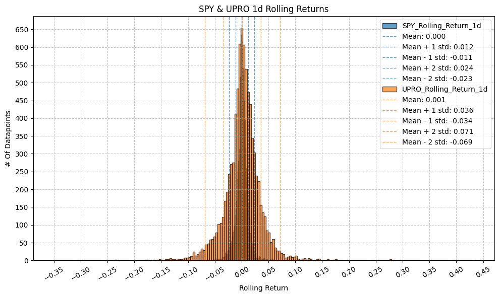
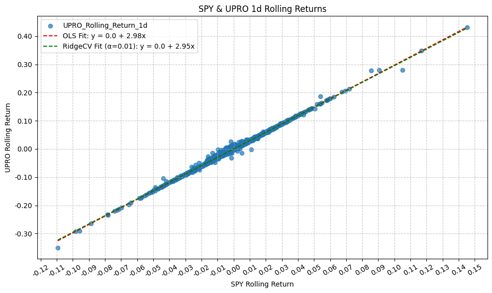
                              OLS Regression Results
==================================================================================
Dep. Variable:     UPRO_Rolling_Return_1d   R-squared:                       0.997
Model:                                OLS   Adj. R-squared:                  0.997
Method:                     Least Squares   F-statistic:                 3.116e+06
Date:                    Mon, 23 Mar 2026   Prob (F-statistic):               0.00
Time:                            22:02:20   Log-Likelihood:                 40846.
No. Observations:                    8341   AIC:                        -8.169e+04
Df Residuals:                        8339   BIC:                        -8.167e+04
Df Model:                               1
Covariance Type:                nonrobust
=========================================================================================
                            coef    std err          t      P>|t|      [0.025      0.975]
-----------------------------------------------------------------------------------------
const                  9.233e-06   1.98e-05      0.466      0.641   -2.96e-05    4.81e-05
SPY_Rolling_Return_1d     2.9758      0.002   1765.119      0.000       2.972       2.979
==============================================================================
Omnibus:                     6872.372   Durbin-Watson:                   2.589
Prob(Omnibus):                  0.000   Jarque-Bera (JB):          4230832.210
Skew:                           2.810   Prob(JB):                         0.00
Kurtosis:                     113.191   Cond. No.                         85.2
==============================================================================

Notes:
[1] Standard Errors assume that the covariance matrix of the errors is correctly specified.
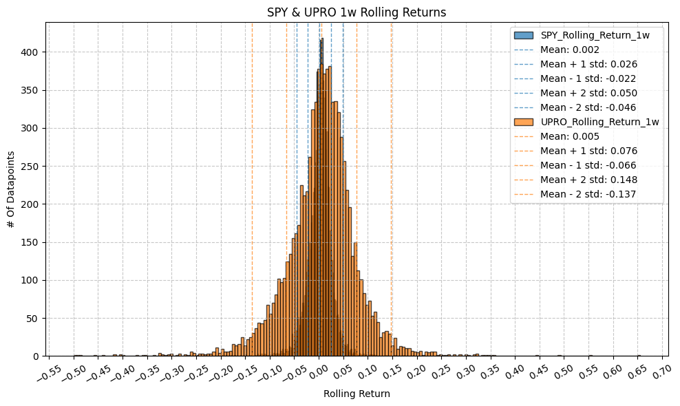
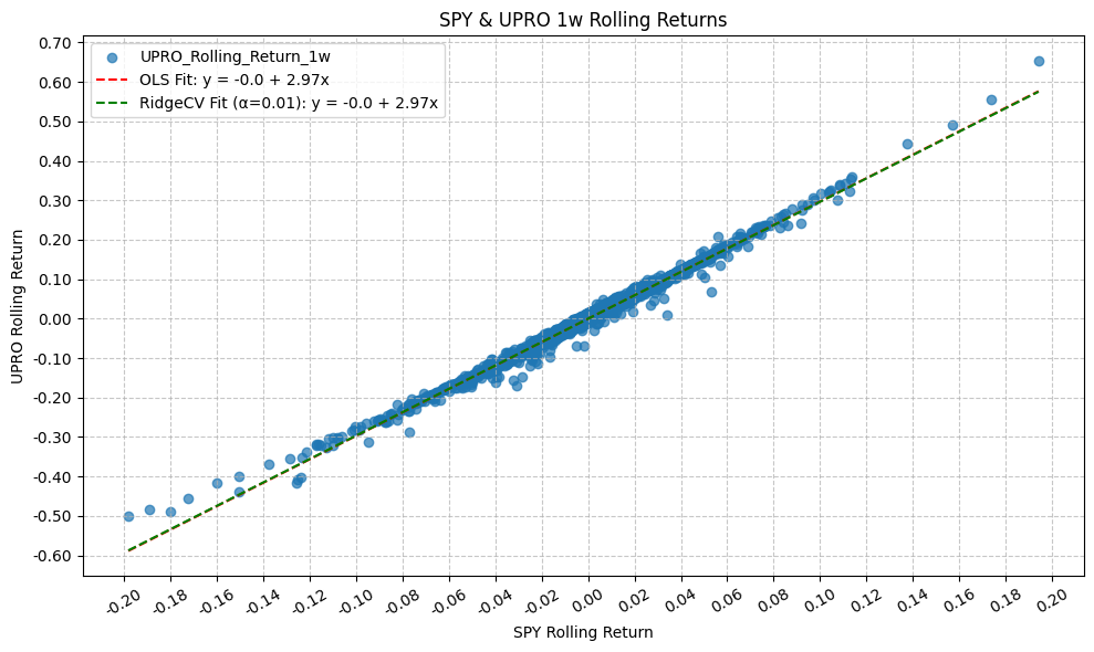
                              OLS Regression Results
==================================================================================
Dep. Variable:     UPRO_Rolling_Return_1w   R-squared:                       0.994
Model:                                OLS   Adj. R-squared:                  0.994
Method:                     Least Squares   F-statistic:                 1.405e+06
Date:                    Mon, 23 Mar 2026   Prob (F-statistic):               0.00
Time:                            22:02:22   Log-Likelihood:                 31615.
No. Observations:                    8337   AIC:                        -6.323e+04
Df Residuals:                        8335   BIC:                        -6.321e+04
Df Model:                               1
Covariance Type:                nonrobust
=========================================================================================
                            coef    std err          t      P>|t|      [0.025      0.975]
-----------------------------------------------------------------------------------------
const                    -0.0003   5.99e-05     -4.291      0.000      -0.000      -0.000
SPY_Rolling_Return_1w     2.9724      0.003   1185.409      0.000       2.967       2.977
==============================================================================
Omnibus:                     3742.727   Durbin-Watson:                   0.955
Prob(Omnibus):                  0.000   Jarque-Bera (JB):          1490835.699
Skew:                          -0.846   Prob(JB):                         0.00
Kurtosis:                      68.489   Cond. No.                         42.0
==============================================================================

Notes:
[1] Standard Errors assume that the covariance matrix of the errors is correctly specified.
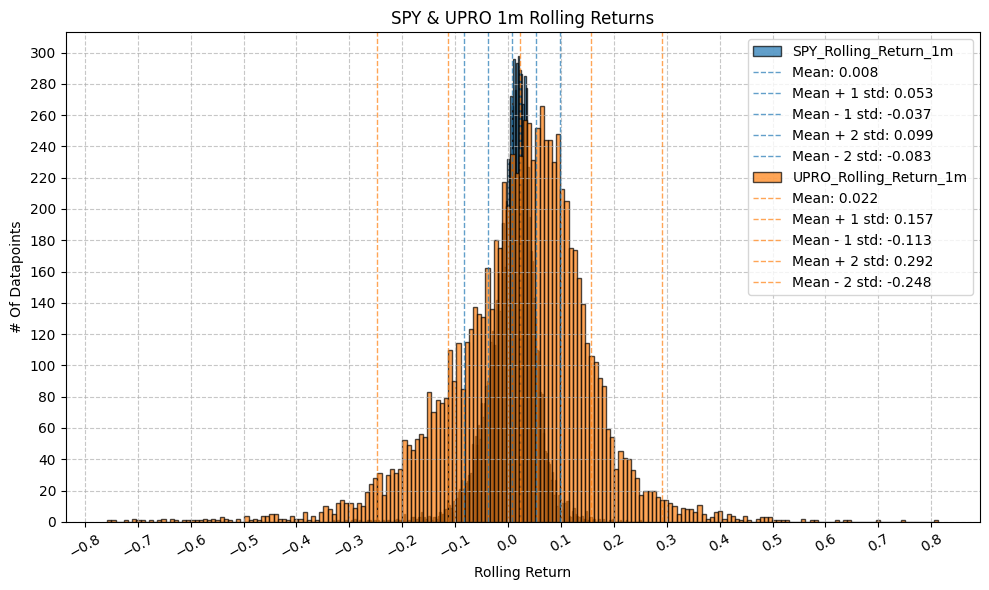
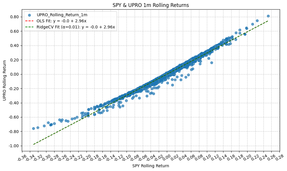
                              OLS Regression Results
==================================================================================
Dep. Variable:     UPRO_Rolling_Return_1m   R-squared:                       0.988
Model:                                OLS   Adj. R-squared:                  0.988
Method:                     Least Squares   F-statistic:                 6.660e+05
Date:                    Mon, 23 Mar 2026   Prob (F-statistic):               0.00
Time:                            22:02:23   Log-Likelihood:                 23146.
No. Observations:                    8321   AIC:                        -4.629e+04
Df Residuals:                        8319   BIC:                        -4.627e+04
Df Model:                               1
Covariance Type:                nonrobust
=========================================================================================
                            coef    std err          t      P>|t|      [0.025      0.975]
-----------------------------------------------------------------------------------------
const                    -0.0015      0.000     -9.057      0.000      -0.002      -0.001
SPY_Rolling_Return_1m     2.9603      0.004    816.112      0.000       2.953       2.967
==============================================================================
Omnibus:                     2880.665   Durbin-Watson:                   0.314
Prob(Omnibus):                  0.000   Jarque-Bera (JB):           856508.368
Skew:                          -0.289   Prob(JB):                         0.00
Kurtosis:                      52.700   Cond. No.                         22.1
==============================================================================

Notes:
[1] Standard Errors assume that the covariance matrix of the errors is correctly specified.
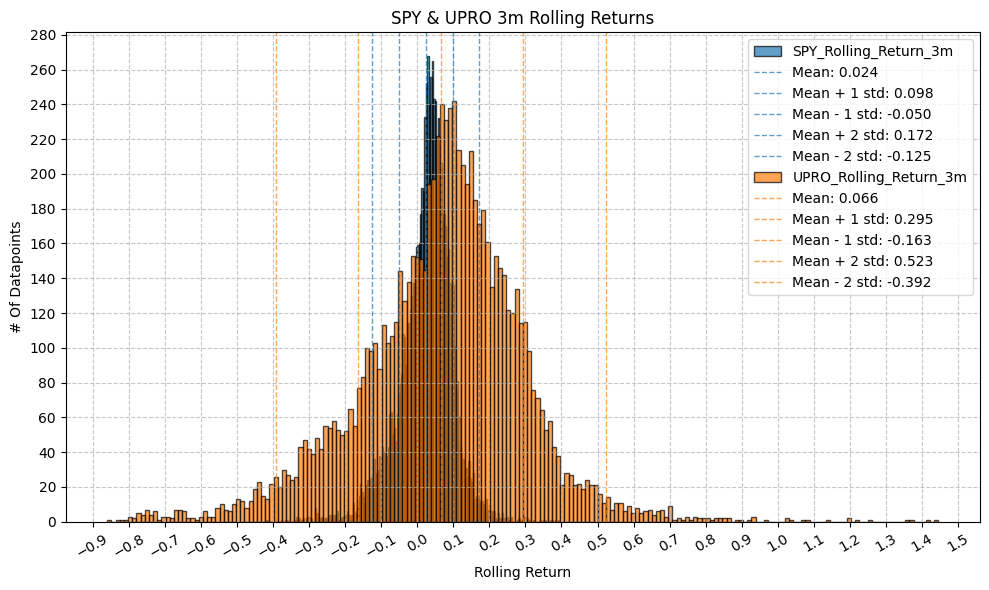
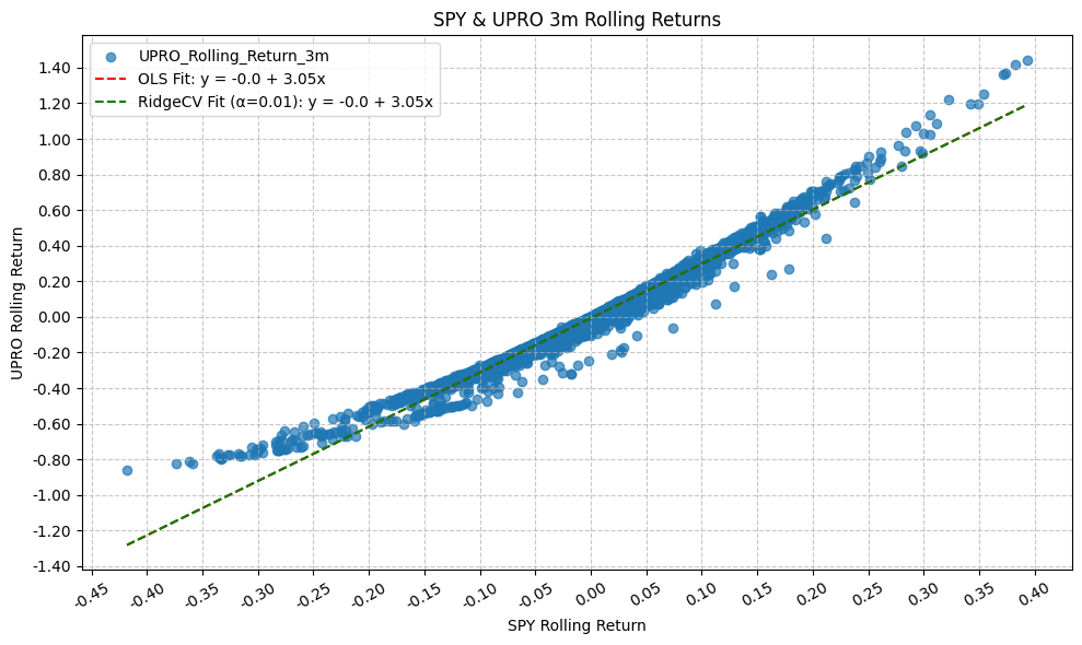
                              OLS Regression Results
==================================================================================
Dep. Variable:     UPRO_Rolling_Return_3m   R-squared:                       0.979
Model:                                OLS   Adj. R-squared:                  0.979
Method:                     Least Squares   F-statistic:                 3.835e+05
Date:                    Mon, 23 Mar 2026   Prob (F-statistic):               0.00
Time:                            22:02:25   Log-Likelihood:                 16431.
No. Observations:                    8279   AIC:                        -3.286e+04
Df Residuals:                        8277   BIC:                        -3.284e+04
Df Model:                               1
Covariance Type:                nonrobust
=========================================================================================
                            coef    std err          t      P>|t|      [0.025      0.975]
-----------------------------------------------------------------------------------------
const                    -0.0068      0.000    -17.760      0.000      -0.008      -0.006
SPY_Rolling_Return_3m     3.0481      0.005    619.270      0.000       3.038       3.058
==============================================================================
Omnibus:                     2415.718   Durbin-Watson:                   0.136
Prob(Omnibus):                  0.000   Jarque-Bera (JB):           133042.469
Skew:                           0.583   Prob(JB):                         0.00
Kurtosis:                      22.604   Cond. No.                         13.5
==============================================================================

Notes:
[1] Standard Errors assume that the covariance matrix of the errors is correctly specified.
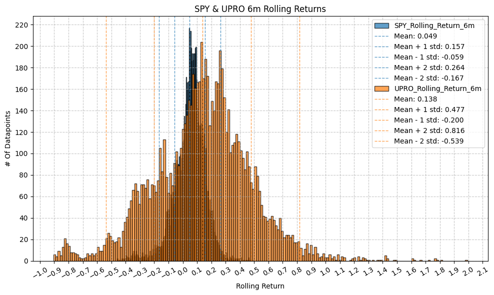
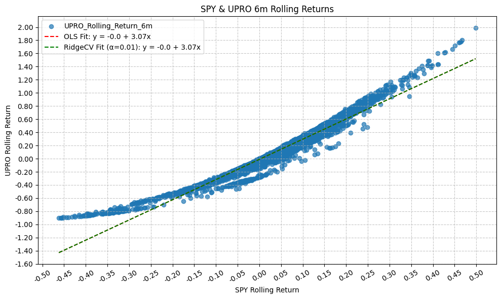
                              OLS Regression Results
==================================================================================
Dep. Variable:     UPRO_Rolling_Return_6m   R-squared:                       0.957
Model:                                OLS   Adj. R-squared:                  0.957
Method:                     Least Squares   F-statistic:                 1.831e+05
Date:                    Mon, 23 Mar 2026   Prob (F-statistic):               0.00
Time:                            22:02:27   Log-Likelihood:                 10169.
No. Observations:                    8216   AIC:                        -2.033e+04
Df Residuals:                        8214   BIC:                        -2.032e+04
Df Model:                               1
Covariance Type:                nonrobust
=========================================================================================
                            coef    std err          t      P>|t|      [0.025      0.975]
-----------------------------------------------------------------------------------------
const                    -0.0110      0.001    -12.928      0.000      -0.013      -0.009
SPY_Rolling_Return_6m     3.0707      0.007    427.893      0.000       3.057       3.085
==============================================================================
Omnibus:                     2069.715   Durbin-Watson:                   0.055
Prob(Omnibus):                  0.000   Jarque-Bera (JB):            26504.206
Skew:                           0.845   Prob(JB):                         0.00
Kurtosis:                      11.635   Cond. No.                         9.29
==============================================================================

Notes:
[1] Standard Errors assume that the covariance matrix of the errors is correctly specified.

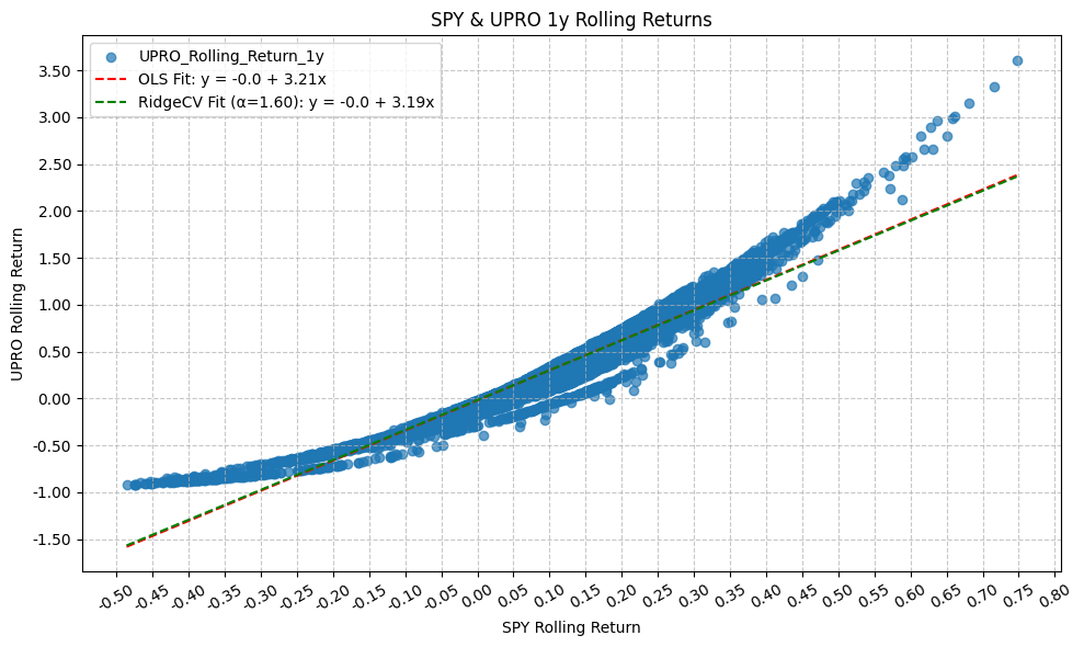
                              OLS Regression Results
==================================================================================
Dep. Variable:     UPRO_Rolling_Return_1y   R-squared:                       0.927
Model:                                OLS   Adj. R-squared:                  0.927
Method:                     Least Squares   F-statistic:                 1.023e+05
Date:                    Mon, 23 Mar 2026   Prob (F-statistic):               0.00
Time:                            22:02:28   Log-Likelihood:                 3934.0
No. Observations:                    8090   AIC:                            -7864.
Df Residuals:                        8088   BIC:                            -7850.
Df Model:                               1
Covariance Type:                nonrobust
=========================================================================================
                            coef    std err          t      P>|t|      [0.025      0.975]
-----------------------------------------------------------------------------------------
const                    -0.0196      0.002    -10.159      0.000      -0.023      -0.016
SPY_Rolling_Return_1y     3.2115      0.010    319.878      0.000       3.192       3.231
==============================================================================
Omnibus:                     1395.388   Durbin-Watson:                   0.031
Prob(Omnibus):                  0.000   Jarque-Bera (JB):             6543.827
Skew:                           0.765   Prob(JB):                         0.00
Kurtosis:                       7.132   Cond. No.                         6.13
==============================================================================

Notes:
[1] Standard Errors assume that the covariance matrix of the errors is correctly specified.
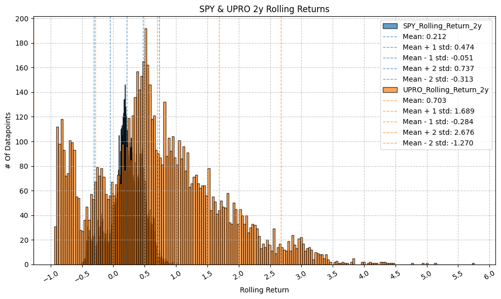
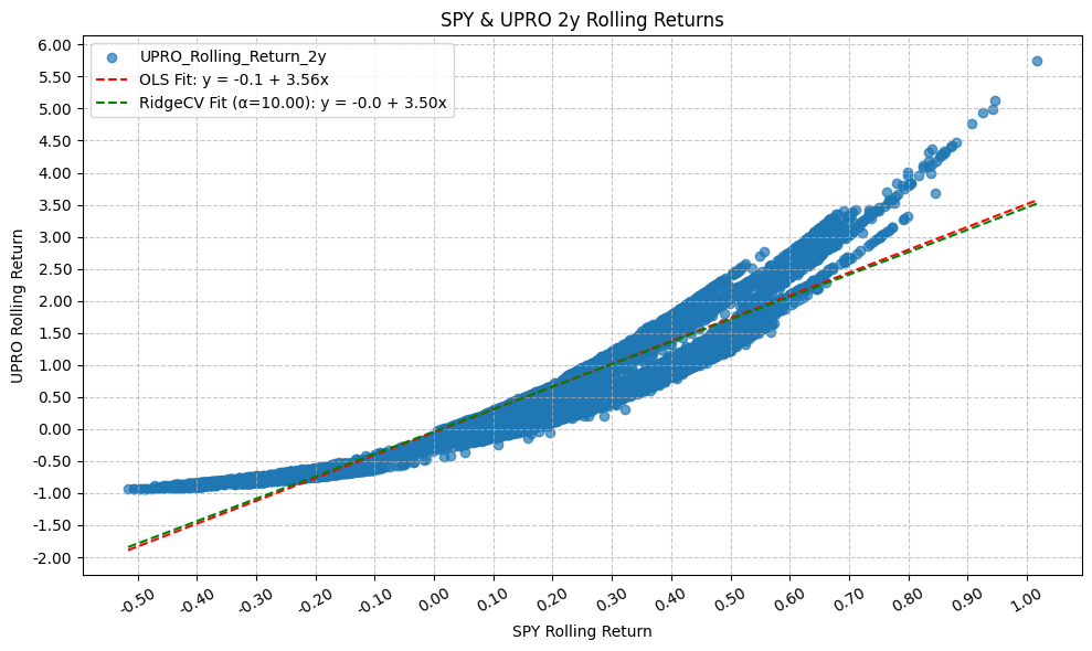
                              OLS Regression Results
==================================================================================
Dep. Variable:     UPRO_Rolling_Return_2y   R-squared:                       0.897
Model:                                OLS   Adj. R-squared:                  0.897
Method:                     Least Squares   F-statistic:                 6.792e+04
Date:                    Mon, 23 Mar 2026   Prob (F-statistic):               0.00
Time:                            22:02:30   Log-Likelihood:                -2124.1
No. Observations:                    7838   AIC:                             4252.
Df Residuals:                        7836   BIC:                             4266.
Df Model:                               1
Covariance Type:                nonrobust
=========================================================================================
                            coef    std err          t      P>|t|      [0.025      0.975]
-----------------------------------------------------------------------------------------
const                    -0.0514      0.005    -11.162      0.000      -0.060      -0.042
SPY_Rolling_Return_2y     3.5609      0.014    260.608      0.000       3.534       3.588
==============================================================================
Omnibus:                      950.451   Durbin-Watson:                   0.018
Prob(Omnibus):                  0.000   Jarque-Bera (JB):             1485.975
Skew:                           0.866   Prob(JB):                         0.00
Kurtosis:                       4.245   Cond. No.                         4.00
==============================================================================

Notes:
[1] Standard Errors assume that the covariance matrix of the errors is correctly specified.
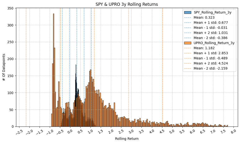
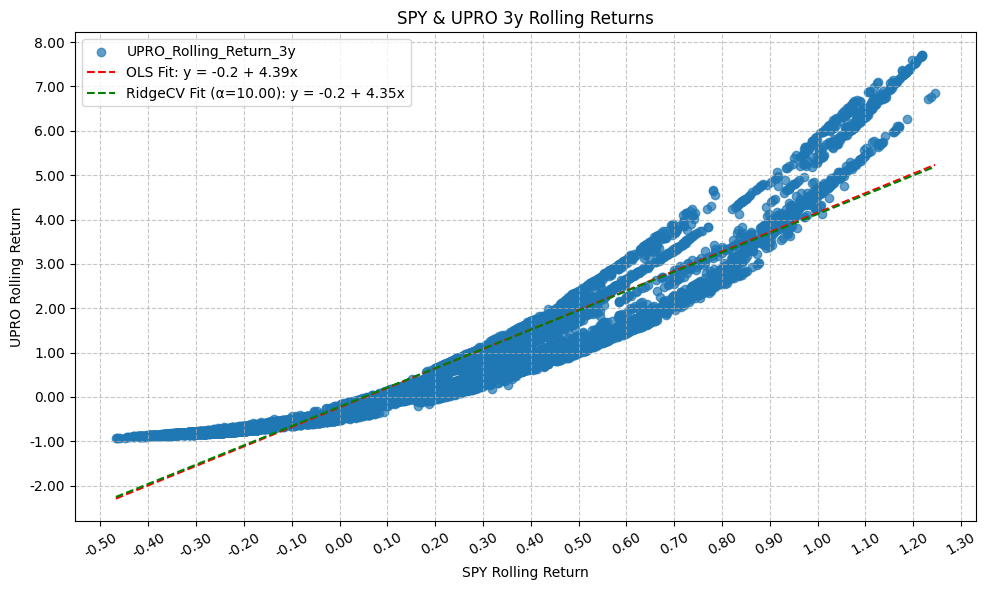
                              OLS Regression Results
==================================================================================
Dep. Variable:     UPRO_Rolling_Return_3y   R-squared:                       0.866
Model:                                OLS   Adj. R-squared:                  0.866
Method:                     Least Squares   F-statistic:                 4.921e+04
Date:                    Mon, 23 Mar 2026   Prob (F-statistic):               0.00
Time:                            22:02:32   Log-Likelihood:                -7020.7
No. Observations:                    7586   AIC:                         1.405e+04
Df Residuals:                        7584   BIC:                         1.406e+04
Df Model:                               1
Covariance Type:                nonrobust
=========================================================================================
                            coef    std err          t      P>|t|      [0.025      0.975]
-----------------------------------------------------------------------------------------
const                    -0.2355      0.009    -24.827      0.000      -0.254      -0.217
SPY_Rolling_Return_3y     4.3908      0.020    221.844      0.000       4.352       4.430
==============================================================================
Omnibus:                     1290.270   Durbin-Watson:                   0.008
Prob(Omnibus):                  0.000   Jarque-Bera (JB):             2447.743
Skew:                           1.054   Prob(JB):                         0.00
Kurtosis:                       4.816   Cond. No.                         3.15
==============================================================================

Notes:
[1] Standard Errors assume that the covariance matrix of the errors is correctly specified.
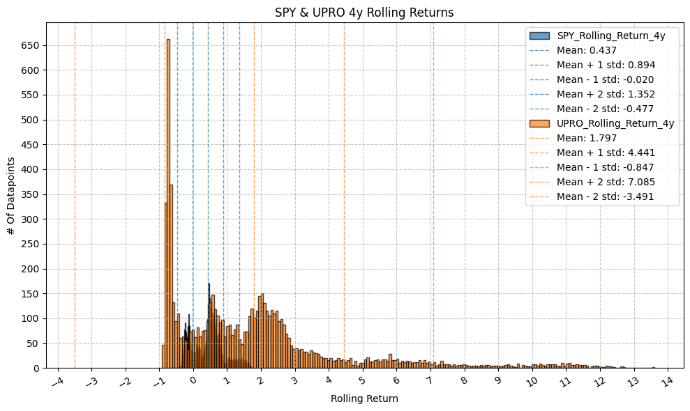
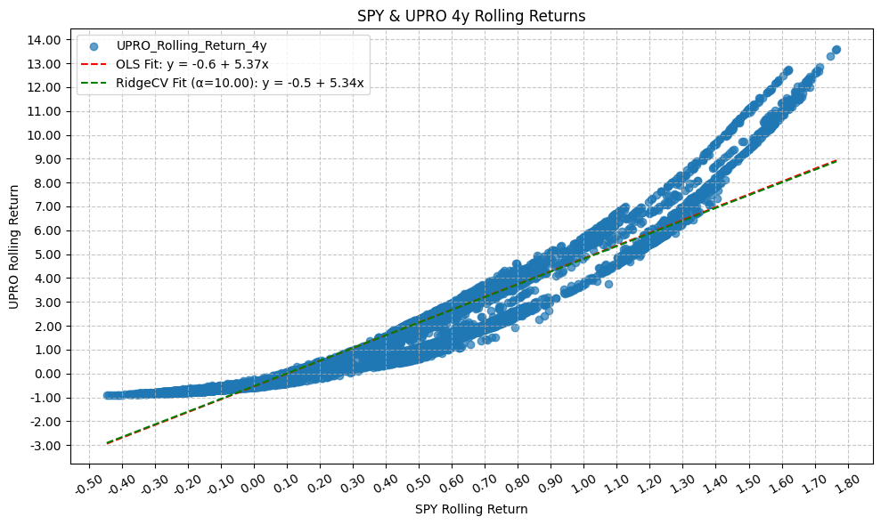
                              OLS Regression Results
==================================================================================
Dep. Variable:     UPRO_Rolling_Return_4y   R-squared:                       0.863
Model:                                OLS   Adj. R-squared:                  0.863
Method:                     Least Squares   F-statistic:                 4.601e+04
Date:                    Mon, 23 Mar 2026   Prob (F-statistic):               0.00
Time:                            22:02:34   Log-Likelihood:                -10260.
No. Observations:                    7334   AIC:                         2.052e+04
Df Residuals:                        7332   BIC:                         2.054e+04
Df Model:                               1
Covariance Type:                nonrobust
=========================================================================================
                            coef    std err          t      P>|t|      [0.025      0.975]
-----------------------------------------------------------------------------------------
const                    -0.5506      0.016    -34.764      0.000      -0.582      -0.520
SPY_Rolling_Return_4y     5.3698      0.025    214.492      0.000       5.321       5.419
==============================================================================
Omnibus:                     1106.304   Durbin-Watson:                   0.008
Prob(Omnibus):                  0.000   Jarque-Bera (JB):             2293.632
Skew:                           0.912   Prob(JB):                         0.00
Kurtosis:                       5.044   Cond. No.                         2.69
==============================================================================

Notes:
[1] Standard Errors assume that the covariance matrix of the errors is correctly specified.
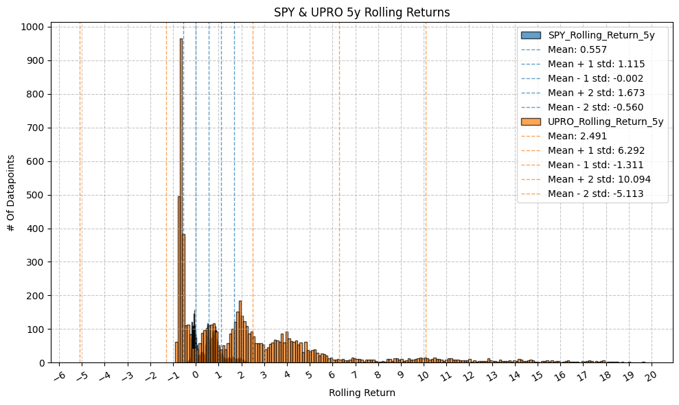
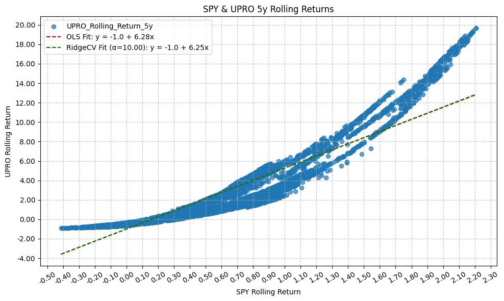
                              OLS Regression Results
==================================================================================
Dep. Variable:     UPRO_Rolling_Return_5y   R-squared:                       0.850
Model:                                OLS   Adj. R-squared:                  0.850
Method:                     Least Squares   F-statistic:                 4.016e+04
Date:                    Mon, 23 Mar 2026   Prob (F-statistic):               0.00
Time:                            22:02:35   Log-Likelihood:                -12785.
No. Observations:                    7082   AIC:                         2.557e+04
Df Residuals:                        7080   BIC:                         2.559e+04
Df Model:                               1
Covariance Type:                nonrobust
=========================================================================================
                            coef    std err          t      P>|t|      [0.025      0.975]
-----------------------------------------------------------------------------------------
const                    -1.0042      0.025    -40.661      0.000      -1.053      -0.956
SPY_Rolling_Return_5y     6.2783      0.031    200.407      0.000       6.217       6.340
==============================================================================
Omnibus:                      686.484   Durbin-Watson:                   0.007
Prob(Omnibus):                  0.000   Jarque-Bera (JB):             1310.280
Skew:                           0.650   Prob(JB):                    2.99e-285
Kurtosis:                       4.658   Cond. No.                         2.51
==============================================================================

Notes:
[1] Standard Errors assume that the covariance matrix of the errors is correctly specified.
Rolling Returns Deviation (SPY & UPRO) #
Next, we will the rolling returns deviation from the expected 3x return for each time period. This will give us a better picture of the volatility decay effect and how it changes over different time horizons.
rolling_returns_stats["Return_Deviation_From_3x"] = rolling_returns_stats["Slope"] - 3.0
pandas_set_decimal_places(3)
display(rolling_returns_stats.set_index("Period"))
| Intercept | Slope | R_Squared | Skew | Average Upside Beta | Average Downside Beta | Asymmetry | Return_Deviation_From_3x | |
|---|---|---|---|---|---|---|---|---|
| Period | ||||||||
| 1d | 0.000 | 2.976 | 0.997 | NaN | 2.939 | NaN | NaN | -0.024 |
| 1w | -0.000 | 2.972 | 0.994 | NaN | 2.757 | NaN | NaN | -0.028 |
| 1m | -0.002 | 2.960 | 0.988 | NaN | 2.494 | -inf | inf | -0.040 |
| 3m | -0.007 | 3.048 | 0.979 | NaN | 2.006 | -inf | inf | 0.048 |
| 6m | -0.011 | 3.071 | 0.957 | NaN | 1.023 | -inf | inf | 0.071 |
| 1y | -0.020 | 3.212 | 0.927 | NaN | 1.640 | -inf | inf | 0.212 |
| 2y | -0.051 | 3.561 | 0.897 | 0.348 | 1.862 | 9.298 | -7.435 | 0.561 |
| 3y | -0.236 | 4.391 | 0.866 | -6.070 | 1.579 | 8.619 | -7.040 | 1.391 |
| 4y | -0.551 | 5.370 | 0.863 | -65.947 | 0.023 | 7.234 | -7.211 | 2.370 |
| 5y | -1.004 | 6.278 | 0.850 | -35.230 | -2.257 | 21.001 | -23.257 | 3.278 |
plot_scatter(
    df=rolling_returns_stats,
    x_plot_column="Period",
    y_plot_columns=["Return_Deviation_From_3x"],
    title="UPRO Deviation from Perfect 3x Leverage by Time Period",
    x_label="Time Period",
    x_format="String",
    x_format_decimal_places=0,
    x_tick_spacing=1,
    x_tick_rotation=0,
    y_label="Deviation from 3x Leverage",
    y_format="Decimal",
    y_format_decimal_places=1,
    y_tick_spacing="Auto",
    y_tick_rotation=0,
    plot_OLS_regression_line=False,
    OLS_column=None,
    plot_Ridge_regression_line=False,
    Ridge_column=None,
    plot_RidgeCV_regression_line=False,
    RidgeCV_column=None,
    regression_constant=False,
    grid=True,
    legend=True,
    export_plot=False,
    plot_file_name=None,
)
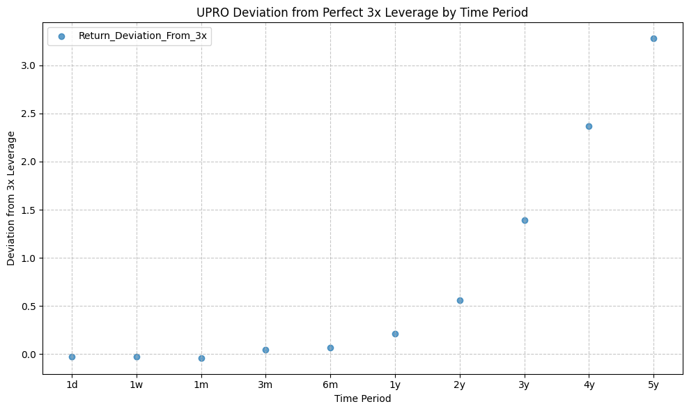
plot_scatter(
    df=rolling_returns_stats,
    x_plot_column="Period",
    y_plot_columns=["Slope"],
    title="UPRO Slope by Time Period",
    x_label="Time Period",
    x_format="String",
    x_format_decimal_places=0,
    x_tick_spacing=1,
    x_tick_rotation=0,
    y_label="Slope",
    y_format="Decimal",
    y_format_decimal_places=1,
    y_tick_spacing="Auto",
    y_tick_rotation=0,
    plot_OLS_regression_line=False,
    OLS_column=None,
    plot_Ridge_regression_line=False,
    Ridge_column=None,
    plot_RidgeCV_regression_line=False,
    RidgeCV_column=None,
    regression_constant=False,
    grid=True,
    legend=True,
    export_plot=False,
    plot_file_name=None,
)
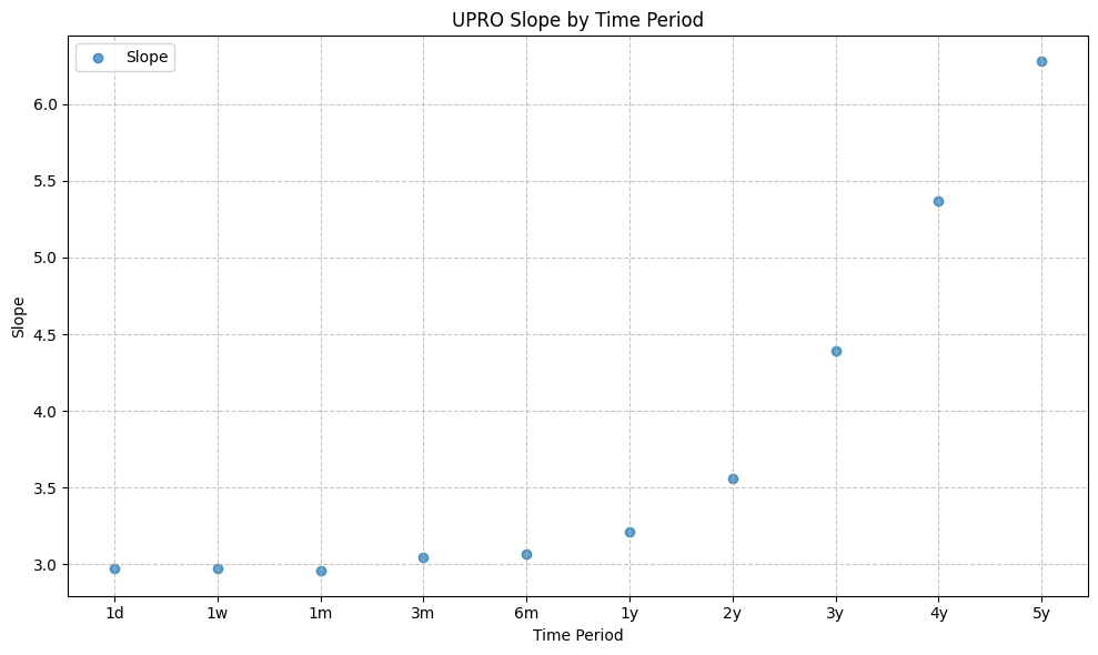
plot_scatter(
    df=rolling_returns_stats,
    x_plot_column="Period",
    y_plot_columns=["Intercept"],
    title="Intercept by Time Period",
    x_label="Time Period",
    x_format="String",
    x_format_decimal_places=0,
    x_tick_spacing=1,
    x_tick_rotation=0,
    y_label="Intercept",
    y_format="Decimal",
    y_format_decimal_places=1,
    y_tick_spacing="Auto",
    y_tick_rotation=0,
    plot_OLS_regression_line=False,
    OLS_column=None,
    plot_Ridge_regression_line=False,
    Ridge_column=None,
    plot_RidgeCV_regression_line=False,
    RidgeCV_column=None,
    regression_constant=False,
    grid=True,
    legend=True,
    export_plot=False,
    plot_file_name=None,
)
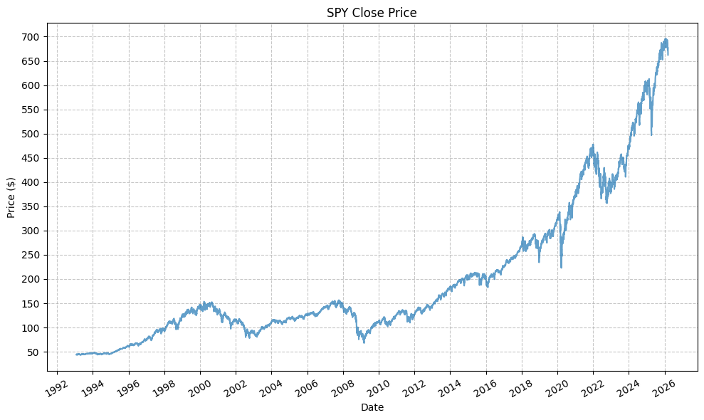
display(rolling_returns_stats.set_index("Period"))
| Intercept | Slope | R_Squared | Skew | Average Upside Beta | Average Downside Beta | Asymmetry | Return_Deviation_From_3x | |
|---|---|---|---|---|---|---|---|---|
| Period | ||||||||
| 1d | 0.000 | 2.976 | 0.997 | NaN | 2.939 | NaN | NaN | -0.024 |
| 1w | -0.000 | 2.972 | 0.994 | NaN | 2.757 | NaN | NaN | -0.028 |
| 1m | -0.002 | 2.960 | 0.988 | NaN | 2.494 | -inf | inf | -0.040 |
| 3m | -0.007 | 3.048 | 0.979 | NaN | 2.006 | -inf | inf | 0.048 |
| 6m | -0.011 | 3.071 | 0.957 | NaN | 1.023 | -inf | inf | 0.071 |
| 1y | -0.020 | 3.212 | 0.927 | NaN | 1.640 | -inf | inf | 0.212 |
| 2y | -0.051 | 3.561 | 0.897 | 0.348 | 1.862 | 9.298 | -7.435 | 0.561 |
| 3y | -0.236 | 4.391 | 0.866 | -6.070 | 1.579 | 8.619 | -7.040 | 1.391 |
| 4y | -0.551 | 5.370 | 0.863 | -65.947 | 0.023 | 7.234 | -7.211 | 2.370 |
| 5y | -1.004 | 6.278 | 0.850 | -35.230 | -2.257 | 21.001 | -23.257 | 3.278 |
Similar as to QQQ/TQQQ, up to 1 year, there is minimal difference between the mean UPRO 1 year rolling return and the hypothetical 3x leverage, with an R^2 of greater than 0.9.
However, as we extend the time period, we see that
- The “leverage factor” increases significantly, resulting in a deviation from the perfect 3x leverage.
- The intercept also begins to deviate significantly from 0.
Rolling Returns Following Drawdowns (SPY & UPRO) #
We will identify the drawdown levels of UPRO and then look at the subsequent rolling returns over various time horizons.
# Copy DataFrame
spy_upro_extrap_future = spy_upro_extrap.copy()

# Create a list of drawdown levels to analyze
drawdown_levels = [-0.10, -0.20, -0.30, -0.40, -0.50, -0.60, -0.70, -0.80, -0.90]

# Shift the rolling return columns by the number of days in the rolling window to get the returns following the drawdown
for etf in etfs:
    for period_name, window in rolling_windows.items():
        spy_upro_extrap_future[f"{etf}_Rolling_Future_Return_{period_name}"] = spy_upro_extrap_future[f"{etf}_Rolling_Return_{period_name}"].shift(-window)
Now, we can analyze the future rolling returns following specific drawdown levels:
# Create a dataframe to hold rolling returns stats
rolling_returns_drawdown_stats = pd.DataFrame()

for drawdown in drawdown_levels:

    for period_name, window in rolling_windows.items():

        try:
            plot_histogram(
                df=spy_upro_extrap_future[spy_upro_extrap_future["UPRO_Drawdown"] <= drawdown],
                plot_columns=[f"SPY_Rolling_Future_Return_{period_name}", f"UPRO_Rolling_Future_Return_{period_name}"],
                title=f"SPY & UPRO {period_name} Rolling Future Returns Post {drawdown} UPRO Drawdown",
                x_label="Rolling Return",
                x_tick_spacing="Auto",
                x_tick_rotation=30,
                y_label="# Of Datapoints",
                y_tick_spacing="Auto",
                y_tick_rotation=0,
                grid=True,
                legend=True,
                export_plot=False,
                plot_file_name=None,
            )

            plot_scatter(
                df=spy_upro_extrap_future[spy_upro_extrap_future["UPRO_Drawdown"] <= drawdown],
                x_plot_column=f"SPY_Rolling_Future_Return_{period_name}",
                y_plot_columns=[f"UPRO_Rolling_Future_Return_{period_name}"],
                title=f"SPY & UPRO {period_name} Rolling Future Returns Post {drawdown} UPRO Drawdown",
                x_label="SPY Rolling Return",
                x_format="Decimal",
                x_format_decimal_places=2,
                x_tick_spacing="Auto",
                x_tick_rotation=30,
                y_label="UPRO Rolling Return",
                y_format="Decimal",
                y_format_decimal_places=2,
                y_tick_spacing="Auto",
                y_tick_rotation=0,
                plot_OLS_regression_line=True,
                OLS_column=f"UPRO_Rolling_Future_Return_{period_name}",
                plot_Ridge_regression_line=False,
                Ridge_column=None,
                plot_RidgeCV_regression_line=True,
                RidgeCV_column=f"UPRO_Rolling_Future_Return_{period_name}",
                regression_constant=True,
                grid=True,
                legend=True,
                export_plot=False,
                plot_file_name=None,
            )

            # Run OLS regression with statsmodels
            model = run_linear_regression(
                df=spy_upro_extrap_future[spy_upro_extrap_future["UPRO_Drawdown"] <= drawdown],
                x_plot_column=f"SPY_Rolling_Future_Return_{period_name}",
                y_plot_column=f"UPRO_Rolling_Future_Return_{period_name}",
                regression_model="OLS-statsmodels",
                regression_constant=True,
            )
            print(model.summary())

            # Filter by drawdown
            drawdown_filter = spy_upro_extrap_future[spy_upro_extrap_future["UPRO_Drawdown"] <= drawdown]

            # Filter by period, drop rows with missing values
            future_filter = drawdown_filter[[f"UPRO_Rolling_Future_Return_{period_name}"]].dropna()

            # Find length of future dataframe
            future_length = len(future_filter)

            # Find length of future dataframe where return is positive
            positive_future_length = len(future_filter[future_filter[f"UPRO_Rolling_Future_Return_{period_name}"] > 0])

            # Calculate percentage of future returns that are positive
            positive_future_percentage = (positive_future_length / future_length) if future_length > 0 else 0

            # Add the regression results to the rolling returns stats dataframe
            intercept = model.params[0]
            # intercept_pvalue = model.pvalues[0]   # p-value for Intercept
            slope = model.params[1]
            # slope_pvalue = model.pvalues[1]       # p-value for Slope
            r_squared = model.rsquared

            rolling_returns_slope_int = pd.DataFrame({
                "Drawdown": drawdown,
                "Period": period_name,
                "Intercept": [intercept],
                # "Intercept_PValue": [intercept_pvalue],
                "Slope": [slope],
                # "Slope_PValue": [slope_pvalue],
                "R_Squared": [r_squared],
                "Positive_Future_Percentage": [positive_future_percentage],
            })

            rolling_returns_drawdown_stats = pd.concat([rolling_returns_drawdown_stats, rolling_returns_slope_int])

        except:
            print(f"Not enough data points for drawdown level {drawdown} and period {period_name} to run regression.")
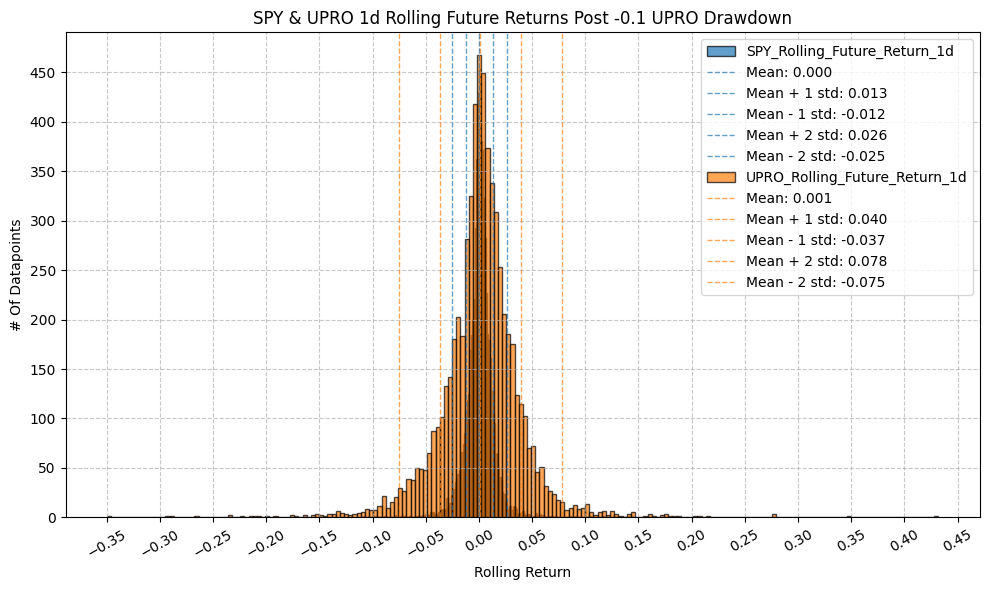

                                  OLS Regression Results
=========================================================================================
Dep. Variable:     UPRO_Rolling_Future_Return_1d   R-squared:                       0.997
Model:                                       OLS   Adj. R-squared:                  0.997
Method:                            Least Squares   F-statistic:                 2.285e+06
Date:                           Mon, 23 Mar 2026   Prob (F-statistic):               0.00
Time:                                   22:02:38   Log-Likelihood:                 29881.
No. Observations:                           6226   AIC:                        -5.976e+04
Df Residuals:                               6224   BIC:                        -5.974e+04
Df Model:                                      1
Covariance Type:                       nonrobust
================================================================================================
                                   coef    std err          t      P>|t|      [0.025      0.975]
------------------------------------------------------------------------------------------------
const                         2.275e-05   2.53e-05      0.900      0.368   -2.68e-05    7.23e-05
SPY_Rolling_Future_Return_1d     2.9763      0.002   1511.487      0.000       2.972       2.980
==============================================================================
Omnibus:                     4602.669   Durbin-Watson:                   2.628
Prob(Omnibus):                  0.000   Jarque-Bera (JB):          2405238.239
Skew:                           2.321   Prob(JB):                         0.00
Kurtosis:                      99.178   Cond. No.                         78.0
==============================================================================

Notes:
[1] Standard Errors assume that the covariance matrix of the errors is correctly specified.


                                  OLS Regression Results
=========================================================================================
Dep. Variable:     UPRO_Rolling_Future_Return_1w   R-squared:                       0.994
Model:                                       OLS   Adj. R-squared:                  0.994
Method:                            Least Squares   F-statistic:                 9.672e+05
Date:                           Mon, 23 Mar 2026   Prob (F-statistic):               0.00
Time:                                   22:02:39   Log-Likelihood:                 22884.
No. Observations:                           6222   AIC:                        -4.576e+04
Df Residuals:                               6220   BIC:                        -4.575e+04
Df Model:                                      1
Covariance Type:                       nonrobust
================================================================================================
                                   coef    std err          t      P>|t|      [0.025      0.975]
------------------------------------------------------------------------------------------------
const                           -0.0002   7.78e-05     -3.048      0.002      -0.000   -8.47e-05
SPY_Rolling_Future_Return_1w     2.9731      0.003    983.448      0.000       2.967       2.979
==============================================================================
Omnibus:                     2735.277   Durbin-Watson:                   0.978
Prob(Omnibus):                  0.000   Jarque-Bera (JB):           782783.199
Skew:                          -0.876   Prob(JB):                         0.00
Kurtosis:                      57.921   Cond. No.                         39.0
==============================================================================

Notes:
[1] Standard Errors assume that the covariance matrix of the errors is correctly specified.
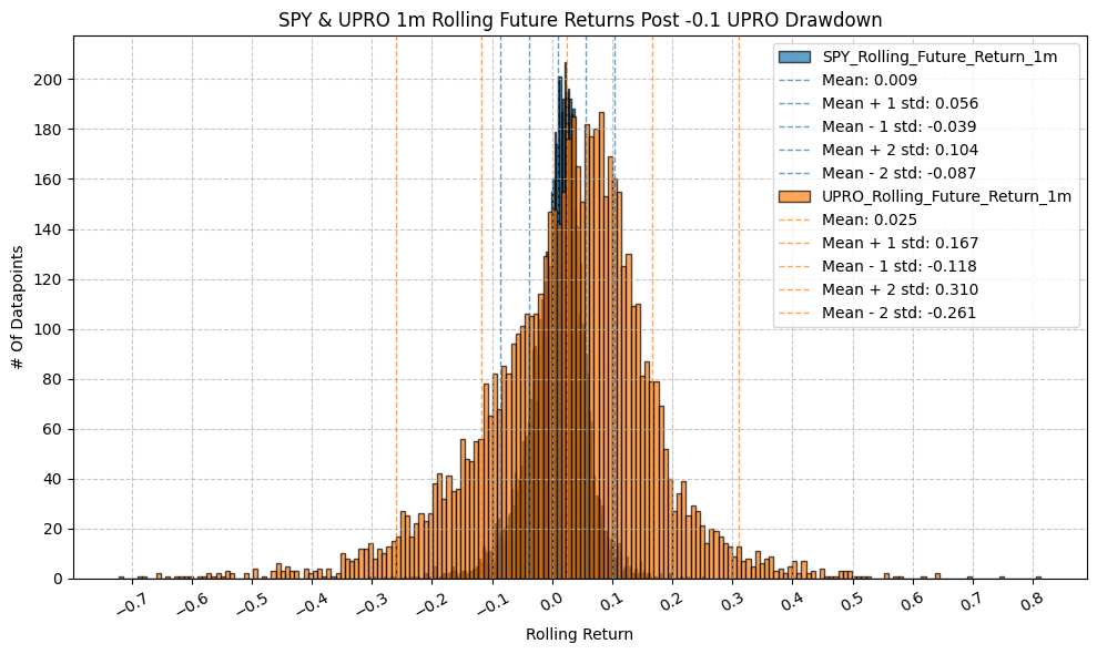

                                  OLS Regression Results
=========================================================================================
Dep. Variable:     UPRO_Rolling_Future_Return_1m   R-squared:                       0.988
Model:                                       OLS   Adj. R-squared:                  0.988
Method:                            Least Squares   F-statistic:                 4.994e+05
Date:                           Mon, 23 Mar 2026   Prob (F-statistic):               0.00
Time:                                   22:02:41   Log-Likelihood:                 16963.
No. Observations:                           6218   AIC:                        -3.392e+04
Df Residuals:                               6216   BIC:                        -3.391e+04
Df Model:                                      1
Covariance Type:                       nonrobust
================================================================================================
                                   coef    std err          t      P>|t|      [0.025      0.975]
------------------------------------------------------------------------------------------------
const                           -0.0015      0.000     -7.180      0.000      -0.002      -0.001
SPY_Rolling_Future_Return_1m     2.9745      0.004    706.672      0.000       2.966       2.983
==============================================================================
Omnibus:                     3370.808   Durbin-Watson:                   0.336
Prob(Omnibus):                  0.000   Jarque-Bera (JB):           387306.157
Skew:                          -1.631   Prob(JB):                         0.00
Kurtosis:                      41.526   Cond. No.                         21.0
==============================================================================

Notes:
[1] Standard Errors assume that the covariance matrix of the errors is correctly specified.
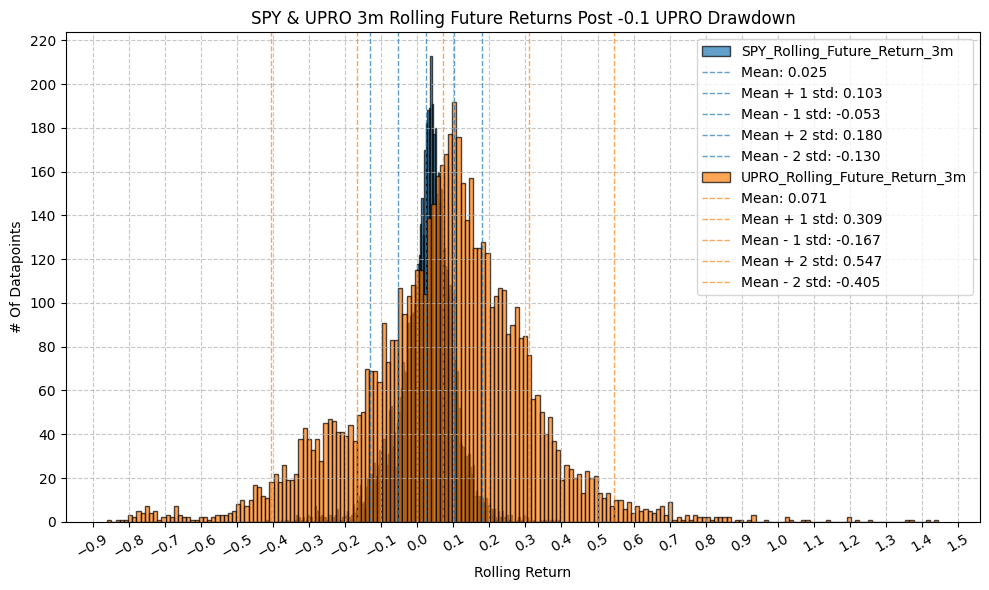

                                  OLS Regression Results
=========================================================================================
Dep. Variable:     UPRO_Rolling_Future_Return_3m   R-squared:                       0.978
Model:                                       OLS   Adj. R-squared:                  0.978
Method:                            Least Squares   F-statistic:                 2.716e+05
Date:                           Mon, 23 Mar 2026   Prob (F-statistic):               0.00
Time:                                   22:02:43   Log-Likelihood:                 11917.
No. Observations:                           6218   AIC:                        -2.383e+04
Df Residuals:                               6216   BIC:                        -2.382e+04
Df Model:                                      1
Covariance Type:                       nonrobust
================================================================================================
                                   coef    std err          t      P>|t|      [0.025      0.975]
------------------------------------------------------------------------------------------------
const                           -0.0048      0.000    -10.056      0.000      -0.006      -0.004
SPY_Rolling_Future_Return_3m     3.0333      0.006    521.172      0.000       3.022       3.045
==============================================================================
Omnibus:                     1724.373   Durbin-Watson:                   0.148
Prob(Omnibus):                  0.000   Jarque-Bera (JB):            87828.721
Skew:                           0.522   Prob(JB):                         0.00
Kurtosis:                      21.382   Cond. No.                         12.9
==============================================================================

Notes:
[1] Standard Errors assume that the covariance matrix of the errors is correctly specified.
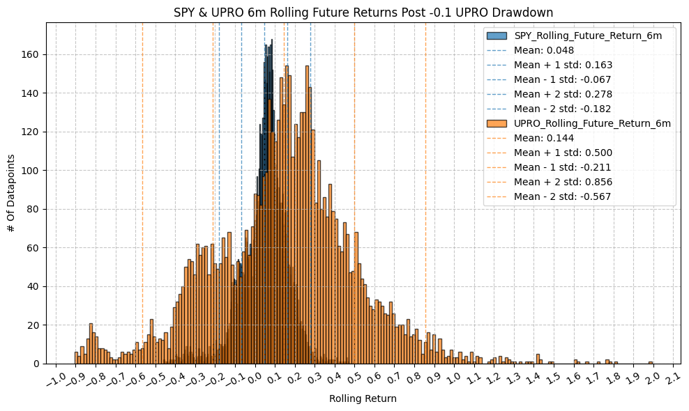

                                  OLS Regression Results
=========================================================================================
Dep. Variable:     UPRO_Rolling_Future_Return_6m   R-squared:                       0.961
Model:                                       OLS   Adj. R-squared:                  0.961
Method:                            Least Squares   F-statistic:                 1.537e+05
Date:                           Mon, 23 Mar 2026   Prob (F-statistic):               0.00
Time:                                   22:02:45   Log-Likelihood:                 7698.8
No. Observations:                           6214   AIC:                        -1.539e+04
Df Residuals:                               6212   BIC:                        -1.538e+04
Df Model:                                      1
Covariance Type:                       nonrobust
================================================================================================
                                   coef    std err          t      P>|t|      [0.025      0.975]
------------------------------------------------------------------------------------------------
const                           -0.0015      0.001     -1.522      0.128      -0.003       0.000
SPY_Rolling_Future_Return_6m     3.0329      0.008    391.995      0.000       3.018       3.048
==============================================================================
Omnibus:                     2086.648   Durbin-Watson:                   0.070
Prob(Omnibus):                  0.000   Jarque-Bera (JB):            20735.224
Skew:                           1.316   Prob(JB):                         0.00
Kurtosis:                      11.553   Cond. No.                         8.72
==============================================================================

Notes:
[1] Standard Errors assume that the covariance matrix of the errors is correctly specified.
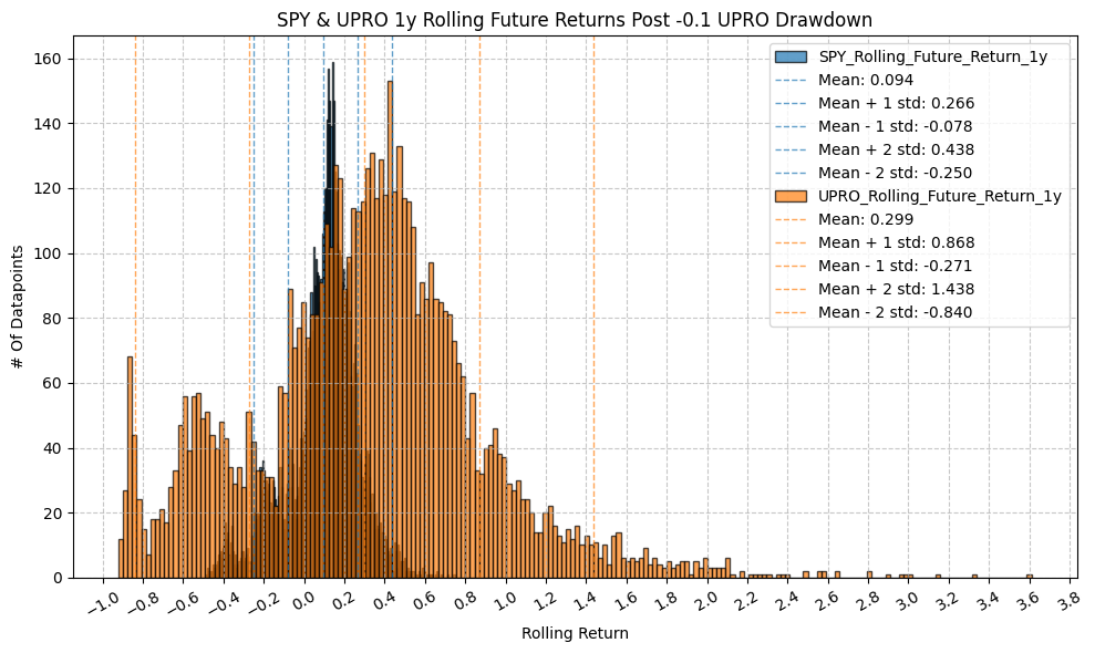
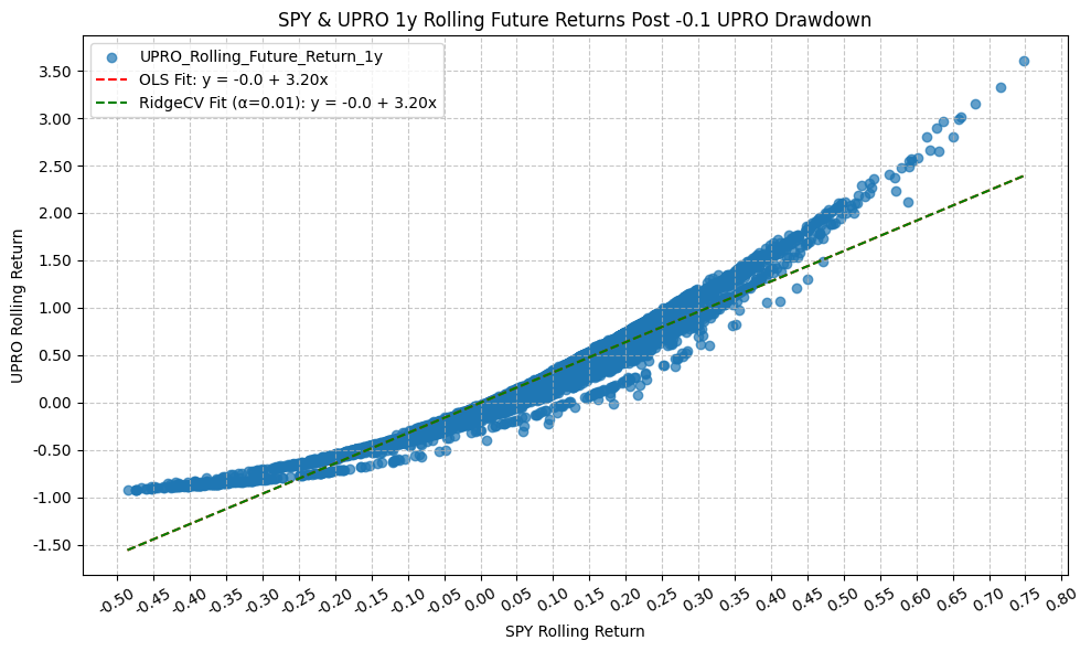
                                  OLS Regression Results
=========================================================================================
Dep. Variable:     UPRO_Rolling_Future_Return_1y   R-squared:                       0.933
Model:                                       OLS   Adj. R-squared:                  0.933
Method:                            Least Squares   F-statistic:                 8.614e+04
Date:                           Mon, 23 Mar 2026   Prob (F-statistic):               0.00
Time:                                   22:02:47   Log-Likelihood:                 3065.5
No. Observations:                           6146   AIC:                            -6127.
Df Residuals:                               6144   BIC:                            -6114.
Df Model:                                      1
Covariance Type:                       nonrobust
================================================================================================
                                   coef    std err          t      P>|t|      [0.025      0.975]
------------------------------------------------------------------------------------------------
const                           -0.0008      0.002     -0.366      0.714      -0.005       0.003
SPY_Rolling_Future_Return_1y     3.1987      0.011    293.494      0.000       3.177       3.220
==============================================================================
Omnibus:                     1575.748   Durbin-Watson:                   0.041
Prob(Omnibus):                  0.000   Jarque-Bera (JB):             7473.065
Skew:                           1.162   Prob(JB):                         0.00
Kurtosis:                       7.877   Cond. No.                         5.87
==============================================================================

Notes:
[1] Standard Errors assume that the covariance matrix of the errors is correctly specified.

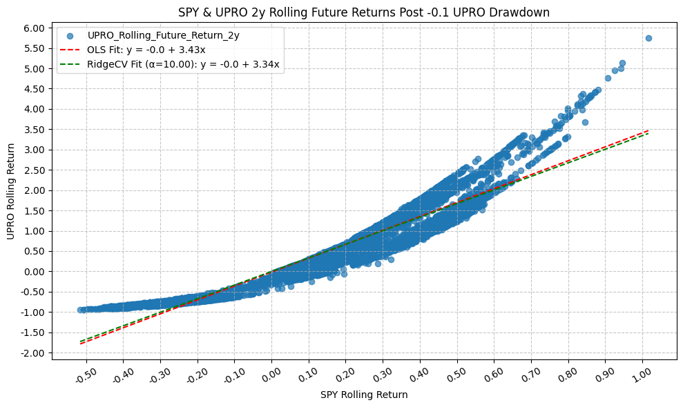
                                  OLS Regression Results
=========================================================================================
Dep. Variable:     UPRO_Rolling_Future_Return_2y   R-squared:                       0.891
Model:                                       OLS   Adj. R-squared:                  0.891
Method:                            Least Squares   F-statistic:                 4.975e+04
Date:                           Mon, 23 Mar 2026   Prob (F-statistic):               0.00
Time:                                   22:02:48   Log-Likelihood:                -1449.4
No. Observations:                           6066   AIC:                             2903.
Df Residuals:                               6064   BIC:                             2916.
Df Model:                                      1
Covariance Type:                       nonrobust
================================================================================================
                                   coef    std err          t      P>|t|      [0.025      0.975]
------------------------------------------------------------------------------------------------
const                           -0.0178      0.005     -3.655      0.000      -0.027      -0.008
SPY_Rolling_Future_Return_2y     3.4265      0.015    223.051      0.000       3.396       3.457
==============================================================================
Omnibus:                     1154.524   Durbin-Watson:                   0.024
Prob(Omnibus):                  0.000   Jarque-Bera (JB):             2672.248
Skew:                           1.077   Prob(JB):                         0.00
Kurtosis:                       5.436   Cond. No.                         4.04
==============================================================================

Notes:
[1] Standard Errors assume that the covariance matrix of the errors is correctly specified.
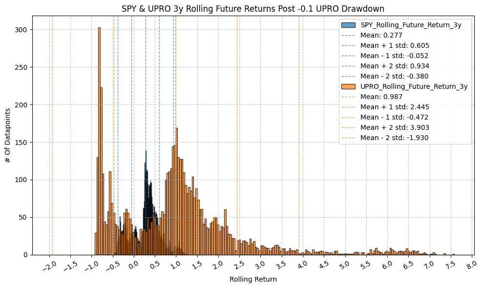
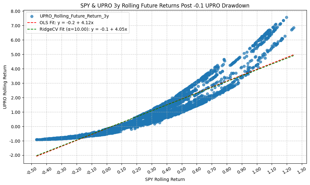
                                  OLS Regression Results
=========================================================================================
Dep. Variable:     UPRO_Rolling_Future_Return_3y   R-squared:                       0.861
Model:                                       OLS   Adj. R-squared:                  0.861
Method:                            Least Squares   F-statistic:                 3.593e+04
Date:                           Mon, 23 Mar 2026   Prob (F-statistic):               0.00
Time:                                   22:02:50   Log-Likelihood:                -4711.2
No. Observations:                           5814   AIC:                             9426.
Df Residuals:                               5812   BIC:                             9440.
Df Model:                                      1
Covariance Type:                       nonrobust
================================================================================================
                                   coef    std err          t      P>|t|      [0.025      0.975]
------------------------------------------------------------------------------------------------
const                           -0.1526      0.009    -16.359      0.000      -0.171      -0.134
SPY_Rolling_Future_Return_3y     4.1182      0.022    189.558      0.000       4.076       4.161
==============================================================================
Omnibus:                     1536.266   Durbin-Watson:                   0.011
Prob(Omnibus):                  0.000   Jarque-Bera (JB):             4893.291
Skew:                           1.338   Prob(JB):                         0.00
Kurtosis:                       6.611   Cond. No.                         3.30
==============================================================================

Notes:
[1] Standard Errors assume that the covariance matrix of the errors is correctly specified.
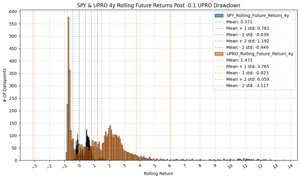
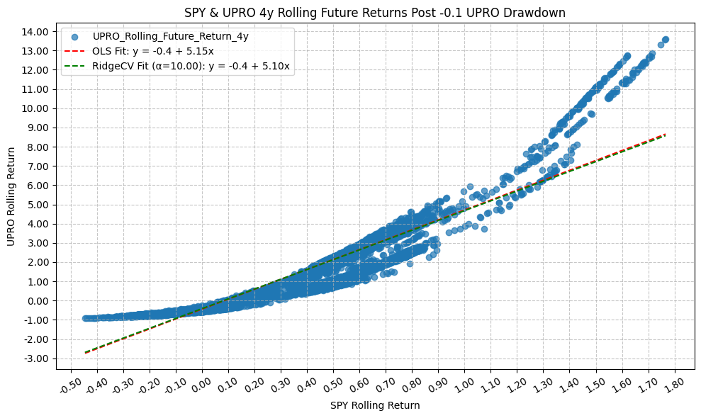
                                  OLS Regression Results
=========================================================================================
Dep. Variable:     UPRO_Rolling_Future_Return_4y   R-squared:                       0.848
Model:                                       OLS   Adj. R-squared:                  0.848
Method:                            Least Squares   F-statistic:                 3.107e+04
Date:                           Mon, 23 Mar 2026   Prob (F-statistic):               0.00
Time:                                   22:02:52   Log-Likelihood:                -7267.4
No. Observations:                           5562   AIC:                         1.454e+04
Df Residuals:                               5560   BIC:                         1.455e+04
Df Model:                                      1
Covariance Type:                       nonrobust
================================================================================================
                                   coef    std err          t      P>|t|      [0.025      0.975]
------------------------------------------------------------------------------------------------
const                           -0.4423      0.016    -27.350      0.000      -0.474      -0.411
SPY_Rolling_Future_Return_4y     5.1509      0.029    176.254      0.000       5.094       5.208
==============================================================================
Omnibus:                     1906.031   Durbin-Watson:                   0.013
Prob(Omnibus):                  0.000   Jarque-Bera (JB):            10147.193
Skew:                           1.552   Prob(JB):                         0.00
Kurtosis:                       8.844   Cond. No.                         2.83
==============================================================================

Notes:
[1] Standard Errors assume that the covariance matrix of the errors is correctly specified.
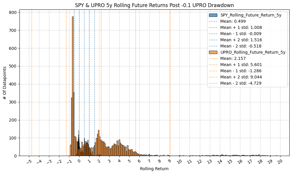
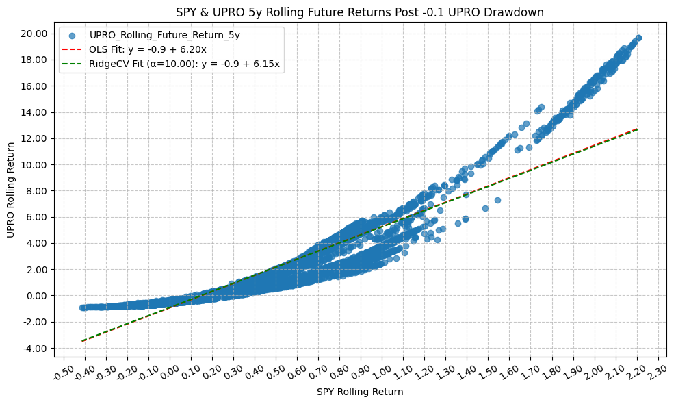
                                  OLS Regression Results
=========================================================================================
Dep. Variable:     UPRO_Rolling_Future_Return_5y   R-squared:                       0.838
Model:                                       OLS   Adj. R-squared:                  0.838
Method:                            Least Squares   F-statistic:                 2.843e+04
Date:                           Mon, 23 Mar 2026   Prob (F-statistic):               0.00
Time:                                   22:02:54   Log-Likelihood:                -9616.6
No. Observations:                           5508   AIC:                         1.924e+04
Df Residuals:                               5506   BIC:                         1.925e+04
Df Model:                                      1
Covariance Type:                       nonrobust
================================================================================================
                                   coef    std err          t      P>|t|      [0.025      0.975]
------------------------------------------------------------------------------------------------
const                           -0.9355      0.026    -35.724      0.000      -0.987      -0.884
SPY_Rolling_Future_Return_5y     6.1974      0.037    168.611      0.000       6.125       6.269
==============================================================================
Omnibus:                     1244.010   Durbin-Watson:                   0.010
Prob(Omnibus):                  0.000   Jarque-Bera (JB):             4368.458
Skew:                           1.109   Prob(JB):                         0.00
Kurtosis:                       6.758   Cond. No.                         2.58
==============================================================================

Notes:
[1] Standard Errors assume that the covariance matrix of the errors is correctly specified.


                                  OLS Regression Results
=========================================================================================
Dep. Variable:     UPRO_Rolling_Future_Return_1d   R-squared:                       0.997
Model:                                       OLS   Adj. R-squared:                  0.997
Method:                            Least Squares   F-statistic:                 1.836e+06
Date:                           Mon, 23 Mar 2026   Prob (F-statistic):               0.00
Time:                                   22:02:56   Log-Likelihood:                 25121.
No. Observations:                           5293   AIC:                        -5.024e+04
Df Residuals:                               5291   BIC:                        -5.023e+04
Df Model:                                      1
Covariance Type:                       nonrobust
================================================================================================
                                   coef    std err          t      P>|t|      [0.025      0.975]
------------------------------------------------------------------------------------------------
const                         3.565e-05   2.89e-05      1.233      0.218    -2.1e-05    9.23e-05
SPY_Rolling_Future_Return_1d     2.9771      0.002   1355.166      0.000       2.973       2.981
==============================================================================
Omnibus:                     3682.841   Durbin-Watson:                   2.648
Prob(Omnibus):                  0.000   Jarque-Bera (JB):          1786814.598
Skew:                           2.082   Prob(JB):                         0.00
Kurtosis:                      92.914   Cond. No.                         76.0
==============================================================================

Notes:
[1] Standard Errors assume that the covariance matrix of the errors is correctly specified.

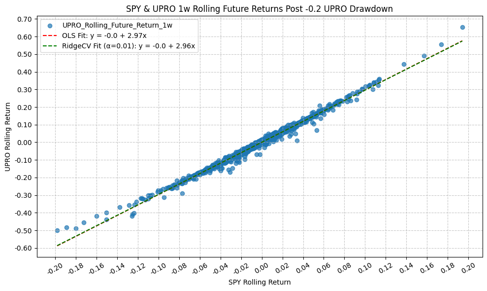
                                  OLS Regression Results
=========================================================================================
Dep. Variable:     UPRO_Rolling_Future_Return_1w   R-squared:                       0.993
Model:                                       OLS   Adj. R-squared:                  0.993
Method:                            Least Squares   F-statistic:                 7.714e+05
Date:                           Mon, 23 Mar 2026   Prob (F-statistic):               0.00
Time:                                   22:02:57   Log-Likelihood:                 19160.
No. Observations:                           5293   AIC:                        -3.832e+04
Df Residuals:                               5291   BIC:                        -3.830e+04
Df Model:                                      1
Covariance Type:                       nonrobust
================================================================================================
                                   coef    std err          t      P>|t|      [0.025      0.975]
------------------------------------------------------------------------------------------------
const                           -0.0002   8.94e-05     -2.238      0.025      -0.000   -2.48e-05
SPY_Rolling_Future_Return_1w     2.9707      0.003    878.290      0.000       2.964       2.977
==============================================================================
Omnibus:                     2332.587   Durbin-Watson:                   0.986
Prob(Omnibus):                  0.000   Jarque-Bera (JB):           564852.970
Skew:                          -0.920   Prob(JB):                         0.00
Kurtosis:                      53.575   Cond. No.                         38.0
==============================================================================

Notes:
[1] Standard Errors assume that the covariance matrix of the errors is correctly specified.
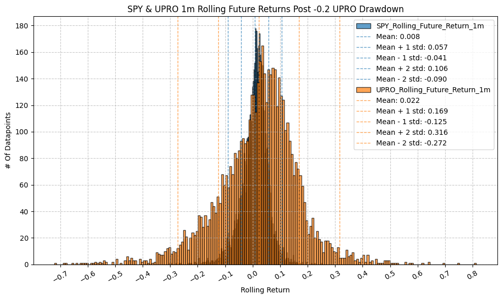

                                  OLS Regression Results
=========================================================================================
Dep. Variable:     UPRO_Rolling_Future_Return_1m   R-squared:                       0.987
Model:                                       OLS   Adj. R-squared:                  0.987
Method:                            Least Squares   F-statistic:                 4.024e+05
Date:                           Mon, 23 Mar 2026   Prob (F-statistic):               0.00
Time:                                   22:02:59   Log-Likelihood:                 14137.
No. Observations:                           5293   AIC:                        -2.827e+04
Df Residuals:                               5291   BIC:                        -2.826e+04
Df Model:                                      1
Covariance Type:                       nonrobust
================================================================================================
                                   coef    std err          t      P>|t|      [0.025      0.975]
------------------------------------------------------------------------------------------------
const                           -0.0014      0.000     -6.029      0.000      -0.002      -0.001
SPY_Rolling_Future_Return_1m     2.9715      0.005    634.383      0.000       2.962       2.981
==============================================================================
Omnibus:                     2856.650   Durbin-Watson:                   0.332
Prob(Omnibus):                  0.000   Jarque-Bera (JB):           280043.841
Skew:                          -1.657   Prob(JB):                         0.00
Kurtosis:                      38.480   Cond. No.                         20.4
==============================================================================

Notes:
[1] Standard Errors assume that the covariance matrix of the errors is correctly specified.
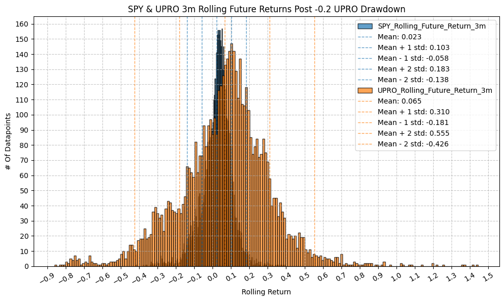

                                  OLS Regression Results
=========================================================================================
Dep. Variable:     UPRO_Rolling_Future_Return_3m   R-squared:                       0.977
Model:                                       OLS   Adj. R-squared:                  0.977
Method:                            Least Squares   F-statistic:                 2.274e+05
Date:                           Mon, 23 Mar 2026   Prob (F-statistic):               0.00
Time:                                   22:03:01   Log-Likelihood:                 9942.5
No. Observations:                           5293   AIC:                        -1.988e+04
Df Residuals:                               5291   BIC:                        -1.987e+04
Df Model:                                      1
Covariance Type:                       nonrobust
================================================================================================
                                   coef    std err          t      P>|t|      [0.025      0.975]
------------------------------------------------------------------------------------------------
const                           -0.0036      0.001     -6.759      0.000      -0.005      -0.003
SPY_Rolling_Future_Return_3m     3.0229      0.006    476.840      0.000       3.010       3.035
==============================================================================
Omnibus:                     1416.059   Durbin-Watson:                   0.159
Prob(Omnibus):                  0.000   Jarque-Bera (JB):            70518.667
Skew:                           0.467   Prob(JB):                         0.00
Kurtosis:                      20.857   Cond. No.                         12.5
==============================================================================

Notes:
[1] Standard Errors assume that the covariance matrix of the errors is correctly specified.
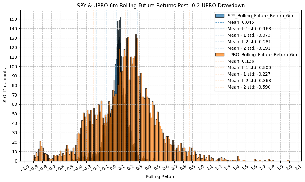
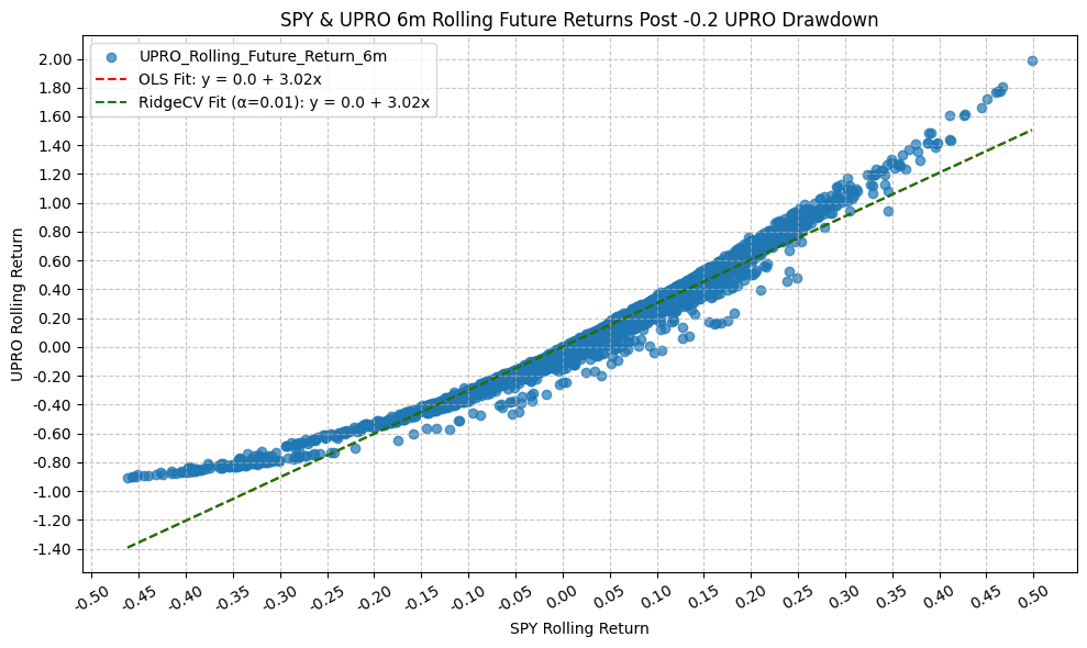
                                  OLS Regression Results
=========================================================================================
Dep. Variable:     UPRO_Rolling_Future_Return_6m   R-squared:                       0.960
Model:                                       OLS   Adj. R-squared:                  0.960
Method:                            Least Squares   F-statistic:                 1.281e+05
Date:                           Mon, 23 Mar 2026   Prob (F-statistic):               0.00
Time:                                   22:03:02   Log-Likelihood:                 6392.5
No. Observations:                           5293   AIC:                        -1.278e+04
Df Residuals:                               5291   BIC:                        -1.277e+04
Df Model:                                      1
Covariance Type:                       nonrobust
================================================================================================
                                   coef    std err          t      P>|t|      [0.025      0.975]
------------------------------------------------------------------------------------------------
const                            0.0016      0.001      1.529      0.126      -0.000       0.004
SPY_Rolling_Future_Return_6m     3.0176      0.008    357.944      0.000       3.001       3.034
==============================================================================
Omnibus:                     1752.000   Durbin-Watson:                   0.078
Prob(Omnibus):                  0.000   Jarque-Bera (JB):            16360.897
Skew:                           1.309   Prob(JB):                         0.00
Kurtosis:                      11.205   Cond. No.                         8.50
==============================================================================

Notes:
[1] Standard Errors assume that the covariance matrix of the errors is correctly specified.
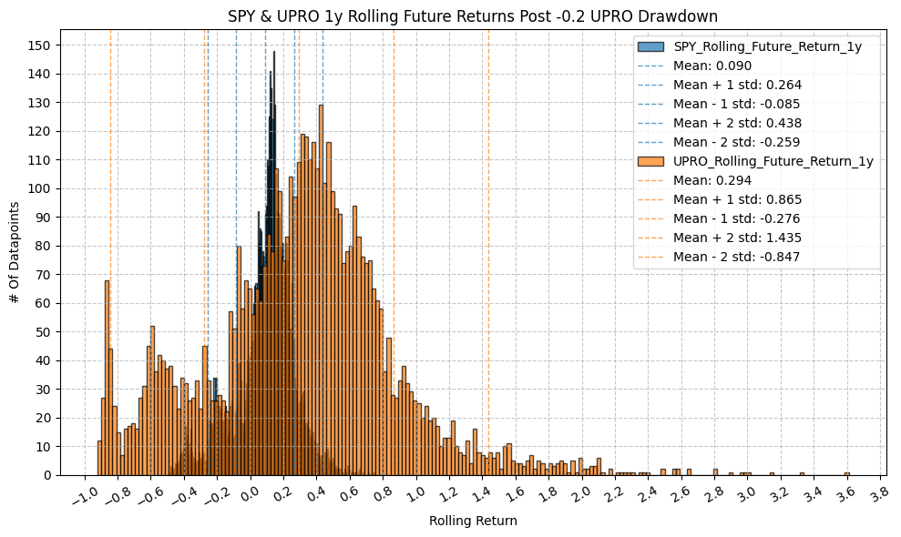
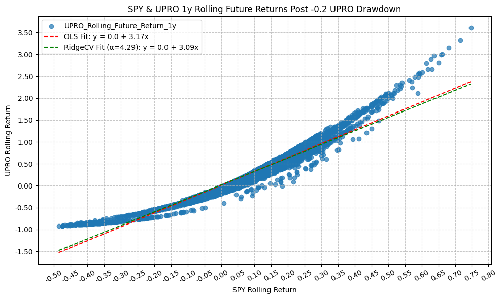
                                  OLS Regression Results
=========================================================================================
Dep. Variable:     UPRO_Rolling_Future_Return_1y   R-squared:                       0.937
Model:                                       OLS   Adj. R-squared:                  0.937
Method:                            Least Squares   F-statistic:                 7.749e+04
Date:                           Mon, 23 Mar 2026   Prob (F-statistic):               0.00
Time:                                   22:03:04   Log-Likelihood:                 2737.5
No. Observations:                           5253   AIC:                            -5471.
Df Residuals:                               5251   BIC:                            -5458.
Df Model:                                      1
Covariance Type:                       nonrobust
================================================================================================
                                   coef    std err          t      P>|t|      [0.025      0.975]
------------------------------------------------------------------------------------------------
const                            0.0100      0.002      4.488      0.000       0.006       0.014
SPY_Rolling_Future_Return_1y     3.1683      0.011    278.372      0.000       3.146       3.191
==============================================================================
Omnibus:                     1724.084   Durbin-Watson:                   0.051
Prob(Omnibus):                  0.000   Jarque-Bera (JB):             9873.553
Skew:                           1.452   Prob(JB):                         0.00
Kurtosis:                       9.056   Cond. No.                         5.79
==============================================================================

Notes:
[1] Standard Errors assume that the covariance matrix of the errors is correctly specified.
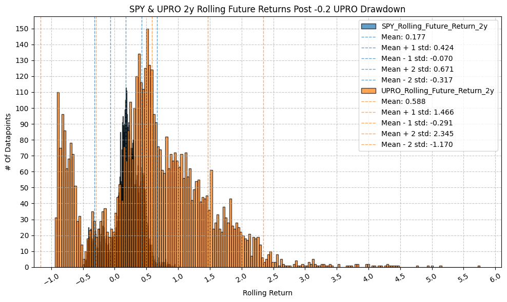
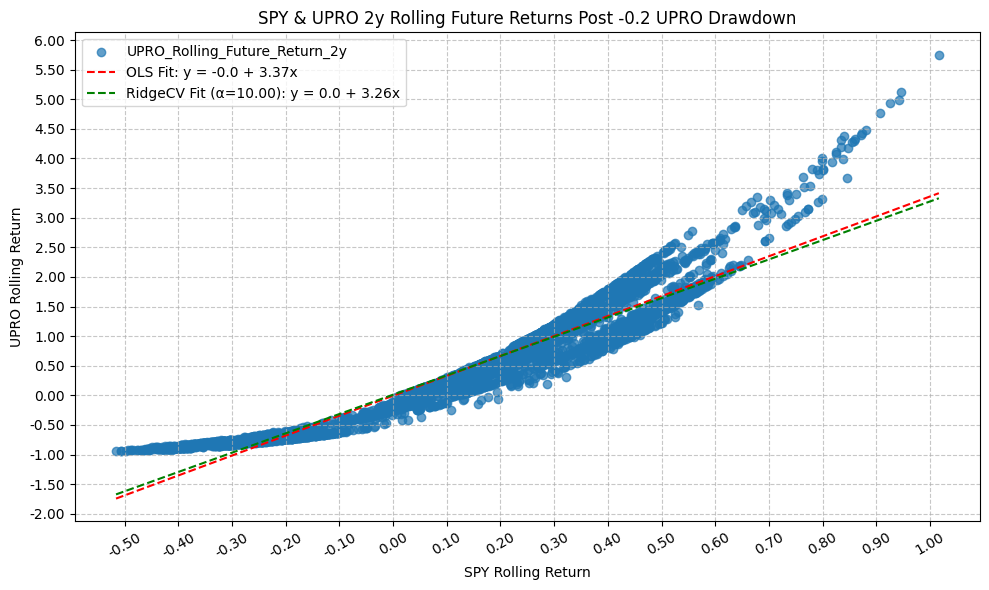
                                  OLS Regression Results
=========================================================================================
Dep. Variable:     UPRO_Rolling_Future_Return_2y   R-squared:                       0.895
Model:                                       OLS   Adj. R-squared:                  0.895
Method:                            Least Squares   F-statistic:                 4.481e+04
Date:                           Mon, 23 Mar 2026   Prob (F-statistic):               0.00
Time:                                   22:03:06   Log-Likelihood:                -840.55
No. Observations:                           5235   AIC:                             1685.
Df Residuals:                               5233   BIC:                             1698.
Df Model:                                      1
Covariance Type:                       nonrobust
================================================================================================
                                   coef    std err          t      P>|t|      [0.025      0.975]
------------------------------------------------------------------------------------------------
const                           -0.0068      0.005     -1.418      0.156      -0.016       0.003
SPY_Rolling_Future_Return_2y     3.3653      0.016    211.680      0.000       3.334       3.396
==============================================================================
Omnibus:                     1350.008   Durbin-Watson:                   0.031
Prob(Omnibus):                  0.000   Jarque-Bera (JB):             4691.598
Skew:                           1.271   Prob(JB):                         0.00
Kurtosis:                       6.879   Cond. No.                         4.18
==============================================================================

Notes:
[1] Standard Errors assume that the covariance matrix of the errors is correctly specified.
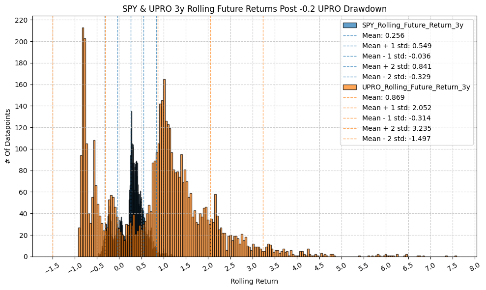
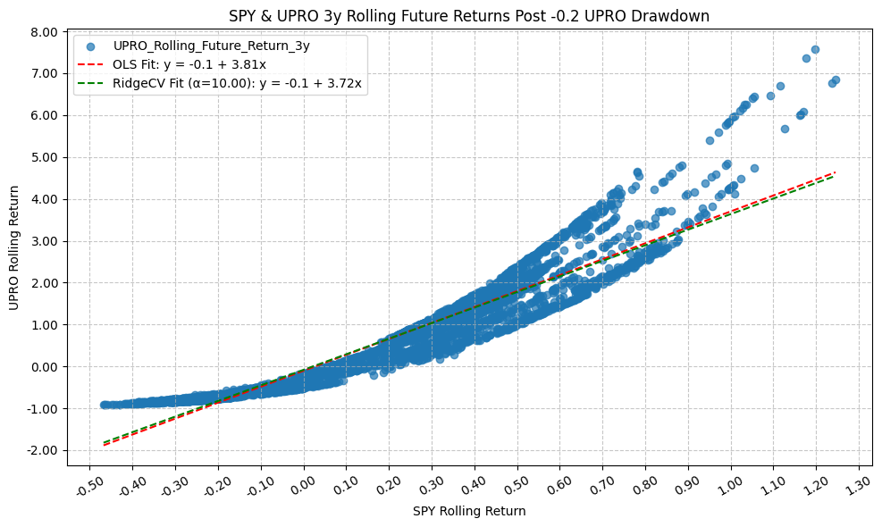
                                  OLS Regression Results
=========================================================================================
Dep. Variable:     UPRO_Rolling_Future_Return_3y   R-squared:                       0.885
Model:                                       OLS   Adj. R-squared:                  0.885
Method:                            Least Squares   F-statistic:                 3.852e+04
Date:                           Mon, 23 Mar 2026   Prob (F-statistic):               0.00
Time:                                   22:03:08   Log-Likelihood:                -2526.9
No. Observations:                           5003   AIC:                             5058.
Df Residuals:                               5001   BIC:                             5071.
Df Model:                                      1
Covariance Type:                       nonrobust
================================================================================================
                                   coef    std err          t      P>|t|      [0.025      0.975]
------------------------------------------------------------------------------------------------
const                           -0.1050      0.008    -13.930      0.000      -0.120      -0.090
SPY_Rolling_Future_Return_3y     3.8056      0.019    196.274      0.000       3.768       3.844
==============================================================================
Omnibus:                     1503.393   Durbin-Watson:                   0.020
Prob(Omnibus):                  0.000   Jarque-Bera (JB):             8255.984
Skew:                           1.327   Prob(JB):                         0.00
Kurtosis:                       8.706   Cond. No.                         3.66
==============================================================================

Notes:
[1] Standard Errors assume that the covariance matrix of the errors is correctly specified.
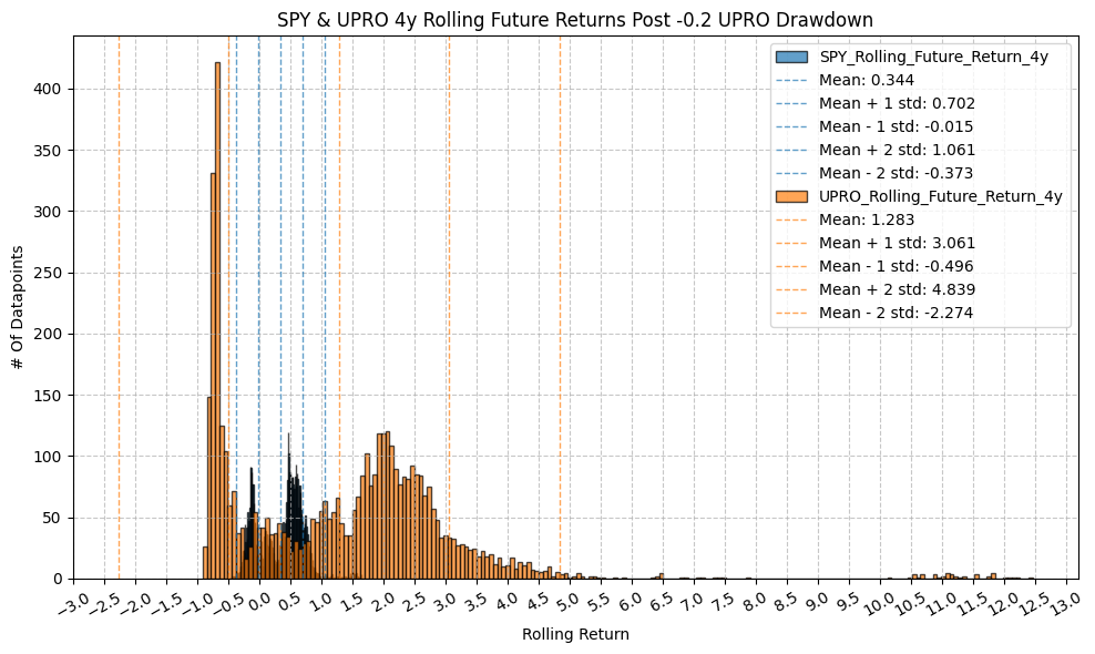
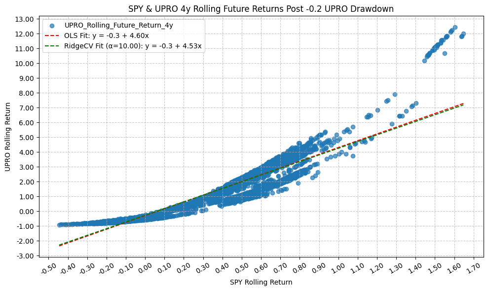
                                  OLS Regression Results
=========================================================================================
Dep. Variable:     UPRO_Rolling_Future_Return_4y   R-squared:                       0.861
Model:                                       OLS   Adj. R-squared:                  0.861
Method:                            Least Squares   F-statistic:                 2.952e+04
Date:                           Mon, 23 Mar 2026   Prob (F-statistic):               0.00
Time:                                   22:03:09   Log-Likelihood:                -4796.4
No. Observations:                           4762   AIC:                             9597.
Df Residuals:                               4760   BIC:                             9610.
Df Model:                                      1
Covariance Type:                       nonrobust
================================================================================================
                                   coef    std err          t      P>|t|      [0.025      0.975]
------------------------------------------------------------------------------------------------
const                           -0.3007      0.013    -22.591      0.000      -0.327      -0.275
SPY_Rolling_Future_Return_4y     4.6041      0.027    171.823      0.000       4.552       4.657
==============================================================================
Omnibus:                     2923.801   Durbin-Watson:                   0.020
Prob(Omnibus):                  0.000   Jarque-Bera (JB):            69358.563
Skew:                           2.506   Prob(JB):                         0.00
Kurtosis:                      21.012   Cond. No.                         3.16
==============================================================================

Notes:
[1] Standard Errors assume that the covariance matrix of the errors is correctly specified.
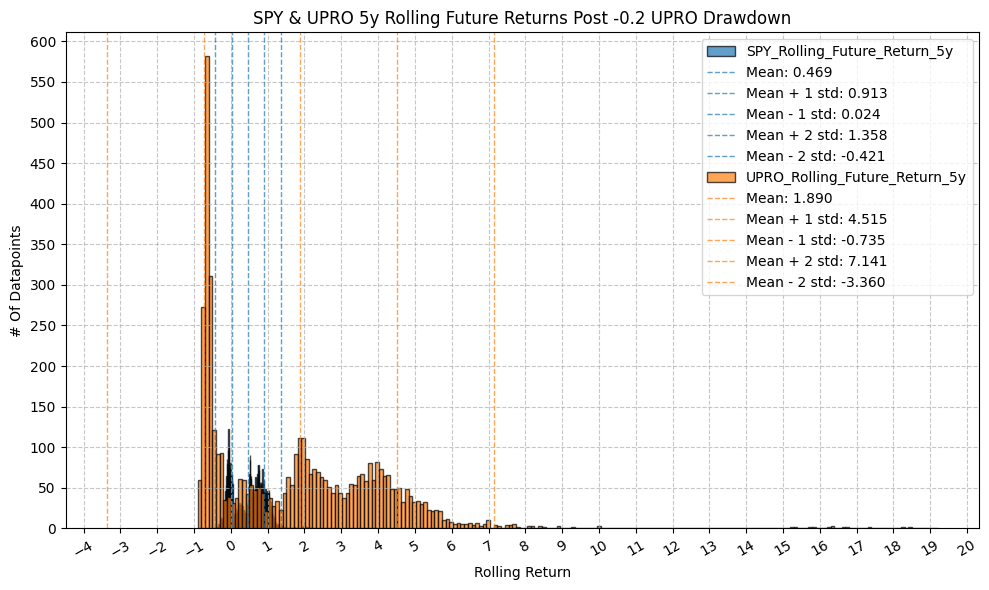
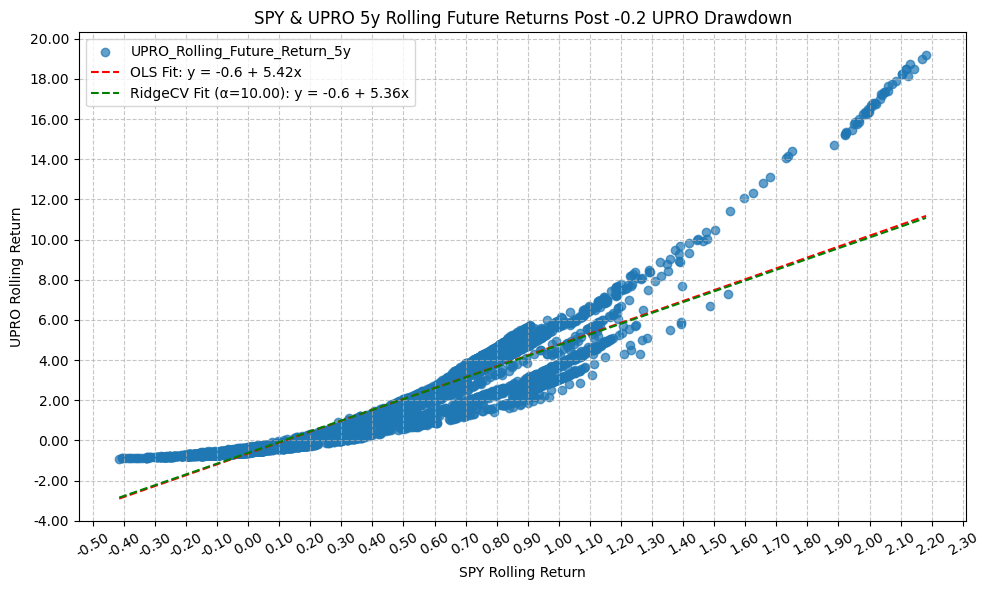
                                  OLS Regression Results
=========================================================================================
Dep. Variable:     UPRO_Rolling_Future_Return_5y   R-squared:                       0.842
Model:                                       OLS   Adj. R-squared:                  0.842
Method:                            Least Squares   F-statistic:                 2.529e+04
Date:                           Mon, 23 Mar 2026   Prob (F-statistic):               0.00
Time:                                   22:03:11   Log-Likelihood:                -6916.0
No. Observations:                           4736   AIC:                         1.384e+04
Df Residuals:                               4734   BIC:                         1.385e+04
Df Model:                                      1
Covariance Type:                       nonrobust
================================================================================================
                                   coef    std err          t      P>|t|      [0.025      0.975]
------------------------------------------------------------------------------------------------
const                           -0.6490      0.022    -29.489      0.000      -0.692      -0.606
SPY_Rolling_Future_Return_5y     5.4199      0.034    159.036      0.000       5.353       5.487
==============================================================================
Omnibus:                     2511.498   Durbin-Watson:                   0.026
Prob(Omnibus):                  0.000   Jarque-Bera (JB):            40921.082
Skew:                           2.156   Prob(JB):                         0.00
Kurtosis:                      16.740   Cond. No.                         2.84
==============================================================================

Notes:
[1] Standard Errors assume that the covariance matrix of the errors is correctly specified.

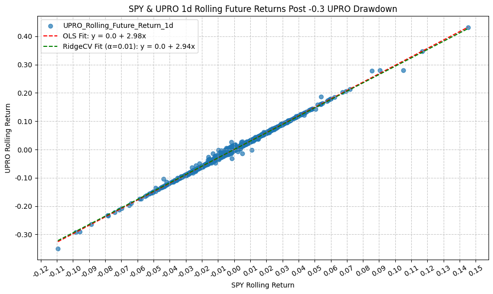
                                  OLS Regression Results
=========================================================================================
Dep. Variable:     UPRO_Rolling_Future_Return_1d   R-squared:                       0.997
Model:                                       OLS   Adj. R-squared:                  0.997
Method:                            Least Squares   F-statistic:                 1.595e+06
Date:                           Mon, 23 Mar 2026   Prob (F-statistic):               0.00
Time:                                   22:03:13   Log-Likelihood:                 22509.
No. Observations:                           4774   AIC:                        -4.501e+04
Df Residuals:                               4772   BIC:                        -4.500e+04
Df Model:                                      1
Covariance Type:                       nonrobust
================================================================================================
                                   coef    std err          t      P>|t|      [0.025      0.975]
------------------------------------------------------------------------------------------------
const                         4.704e-05   3.14e-05      1.498      0.134   -1.45e-05       0.000
SPY_Rolling_Future_Return_1d     2.9767      0.002   1263.047      0.000       2.972       2.981
==============================================================================
Omnibus:                     3250.997   Durbin-Watson:                   2.668
Prob(Omnibus):                  0.000   Jarque-Bera (JB):          1510901.173
Skew:                           2.005   Prob(JB):                         0.00
Kurtosis:                      90.061   Cond. No.                         75.1
==============================================================================

Notes:
[1] Standard Errors assume that the covariance matrix of the errors is correctly specified.
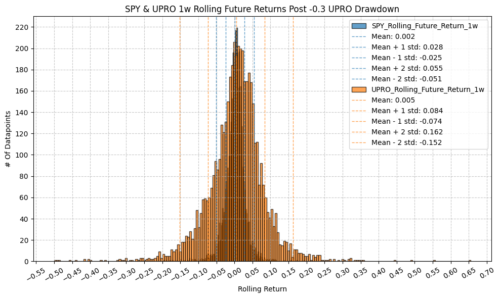

                                  OLS Regression Results
=========================================================================================
Dep. Variable:     UPRO_Rolling_Future_Return_1w   R-squared:                       0.993
Model:                                       OLS   Adj. R-squared:                  0.993
Method:                            Least Squares   F-statistic:                 6.656e+05
Date:                           Mon, 23 Mar 2026   Prob (F-statistic):               0.00
Time:                                   22:03:14   Log-Likelihood:                 17170.
No. Observations:                           4774   AIC:                        -3.434e+04
Df Residuals:                               4772   BIC:                        -3.432e+04
Df Model:                                      1
Covariance Type:                       nonrobust
================================================================================================
                                   coef    std err          t      P>|t|      [0.025      0.975]
------------------------------------------------------------------------------------------------
const                           -0.0002   9.63e-05     -1.927      0.054      -0.000    3.23e-06
SPY_Rolling_Future_Return_1w     2.9715      0.004    815.813      0.000       2.964       2.979
==============================================================================
Omnibus:                     1997.245   Durbin-Watson:                   0.986
Prob(Omnibus):                  0.000   Jarque-Bera (JB):           483280.165
Skew:                          -0.802   Prob(JB):                         0.00
Kurtosis:                      52.264   Cond. No.                         37.9
==============================================================================

Notes:
[1] Standard Errors assume that the covariance matrix of the errors is correctly specified.


                                  OLS Regression Results
=========================================================================================
Dep. Variable:     UPRO_Rolling_Future_Return_1m   R-squared:                       0.987
Model:                                       OLS   Adj. R-squared:                  0.987
Method:                            Least Squares   F-statistic:                 3.515e+05
Date:                           Mon, 23 Mar 2026   Prob (F-statistic):               0.00
Time:                                   22:03:16   Log-Likelihood:                 12680.
No. Observations:                           4774   AIC:                        -2.536e+04
Df Residuals:                               4772   BIC:                        -2.534e+04
Df Model:                                      1
Covariance Type:                       nonrobust
================================================================================================
                                   coef    std err          t      P>|t|      [0.025      0.975]
------------------------------------------------------------------------------------------------
const                           -0.0011      0.000     -4.424      0.000      -0.002      -0.001
SPY_Rolling_Future_Return_1m     2.9620      0.005    592.901      0.000       2.952       2.972
==============================================================================
Omnibus:                     2676.846   Durbin-Watson:                   0.336
Prob(Omnibus):                  0.000   Jarque-Bera (JB):           262764.658
Skew:                          -1.763   Prob(JB):                         0.00
Kurtosis:                      39.174   Cond. No.                         20.3
==============================================================================

Notes:
[1] Standard Errors assume that the covariance matrix of the errors is correctly specified.
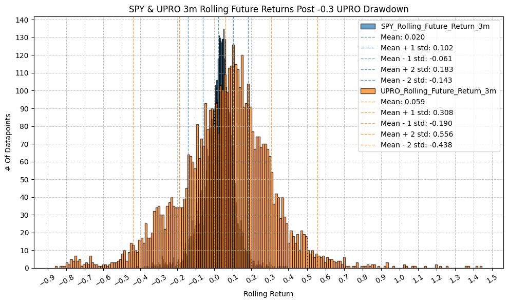
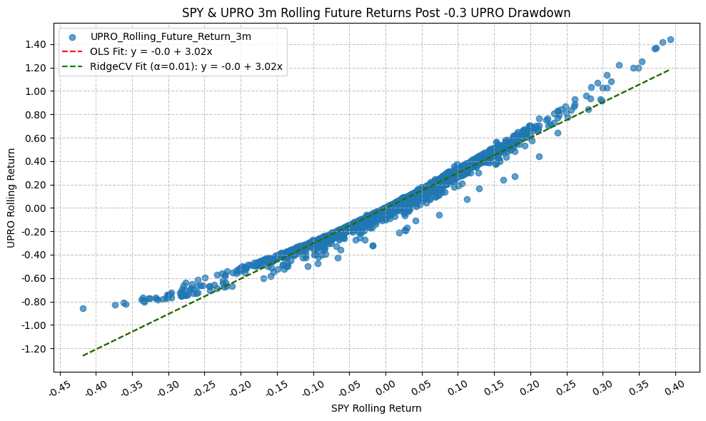
OLS Regression Results
=========================================================================================
Dep. Variable: UPRO_Rolling_Future_Return_3m R-squared: 0.978
Model: OLS Adj. R-squared: 0.978
Method: Least Squares F-statistic: 2.123e+05
Date: Mon, 23 Mar 2026 Prob (F-statistic): 0.00
Time: 22:03:18 Log-Likelihood: 8982.3
No. Observations: 4774 AIC: -1.796e+04
Df Residuals: 4772 BIC: -1.795e+04
Df Model: 1
Covariance Type: nonrobust
================================================================================================
coef std err t P>|t| [0.025 0.975]
------------------------------------------------------------------------------------------------
const -0.0024 0.001 -4.434 0.000 -0.004 -0.001
SPY_Rolling_Future_Return_3m 3.0170 0.007 460.799 0.000 3.004 3.030
==============================================================================
Omnibus: 1428.856 Durbin-Watson: 0.169
Prob(Omnibus): 0.000 Jarque-Bera (JB): 68279.326
Skew: 0.660 Prob(JB): 0.00
Kurtosis: 21.480 Cond. No. 12.3
==============================================================================
Notes:
[1] Standard Errors assume that the covariance matrix of the errors is correctly specified.
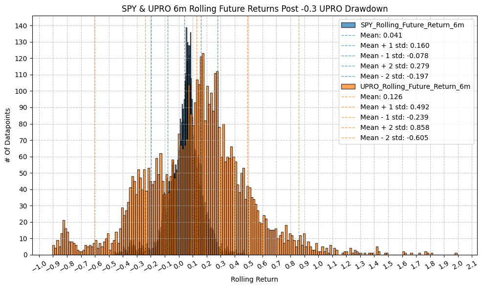

OLS Regression Results
=========================================================================================
Dep. Variable: UPRO_Rolling_Future_Return_6m R-squared: 0.960
Model: OLS Adj. R-squared: 0.960
Method: Least Squares F-statistic: 1.138e+05
Date: Mon, 23 Mar 2026 Prob (F-statistic): 0.00
Time: 22:03:19 Log-Likelihood: 5697.2
No. Observations: 4774 AIC: -1.139e+04
Df Residuals: 4772 BIC: -1.138e+04
Df Model: 1
Covariance Type: nonrobust
================================================================================================
coef std err t P>|t| [0.025 0.975]
------------------------------------------------------------------------------------------------
const 0.0029 0.001 2.546 0.011 0.001 0.005
SPY_Rolling_Future_Return_6m 3.0134 0.009 337.352 0.000 2.996 3.031
==============================================================================
Omnibus: 1652.279 Durbin-Watson: 0.081
Prob(Omnibus): 0.000 Jarque-Bera (JB): 14594.802
Skew: 1.398 Prob(JB): 0.00
Kurtosis: 11.096 Cond. No. 8.43
==============================================================================
Notes:
[1] Standard Errors assume that the covariance matrix of the errors is correctly specified.
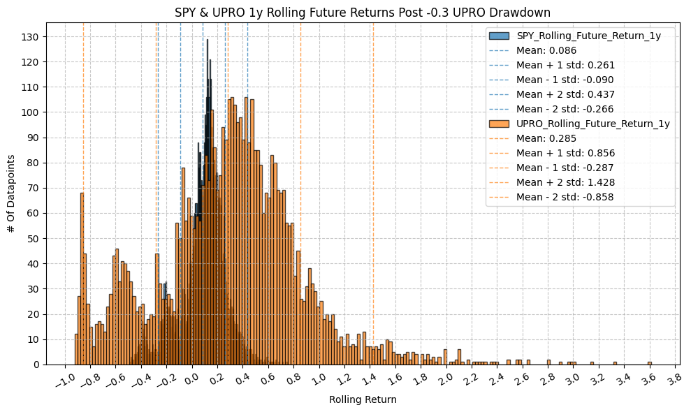

OLS Regression Results
=========================================================================================
Dep. Variable: UPRO_Rolling_Future_Return_1y R-squared: 0.937
Model: OLS Adj. R-squared: 0.937
Method: Least Squares F-statistic: 7.059e+04
Date: Mon, 23 Mar 2026 Prob (F-statistic): 0.00
Time: 22:03:21 Log-Likelihood: 2483.6
No. Observations: 4753 AIC: -4963.
Df Residuals: 4751 BIC: -4950.
Df Model: 1
Covariance Type: nonrobust
================================================================================================
coef std err t P>|t| [0.025 0.975]
------------------------------------------------------------------------------------------------
const 0.0150 0.002 6.479 0.000 0.010 0.020
SPY_Rolling_Future_Return_1y 3.1487 0.012 265.682 0.000 3.125 3.172
==============================================================================
Omnibus: 1666.224 Durbin-Watson: 0.054
Prob(Omnibus): 0.000 Jarque-Bera (JB): 10579.245
Skew: 1.528 Prob(JB): 0.00
Kurtosis: 9.639 Cond. No. 5.74
==============================================================================
Notes:
[1] Standard Errors assume that the covariance matrix of the errors is correctly specified.


OLS Regression Results
=========================================================================================
Dep. Variable: UPRO_Rolling_Future_Return_2y R-squared: 0.901
Model: OLS Adj. R-squared: 0.901
Method: Least Squares F-statistic: 4.347e+04
Date: Mon, 23 Mar 2026 Prob (F-statistic): 0.00
Time: 22:03:23 Log-Likelihood: -568.42
No. Observations: 4753 AIC: 1141.
Df Residuals: 4751 BIC: 1154.
Df Model: 1
Covariance Type: nonrobust
================================================================================================
coef std err t P>|t| [0.025 0.975]
------------------------------------------------------------------------------------------------
const 0.0020 0.005 0.411 0.681 -0.008 0.012
SPY_Rolling_Future_Return_2y 3.3735 0.016 208.485 0.000 3.342 3.405
==============================================================================
Omnibus: 1332.952 Durbin-Watson: 0.031
Prob(Omnibus): 0.000 Jarque-Bera (JB): 5113.406
Skew: 1.349 Prob(JB): 0.00
Kurtosis: 7.306 Cond. No. 4.22
==============================================================================
Notes:
[1] Standard Errors assume that the covariance matrix of the errors is correctly specified.
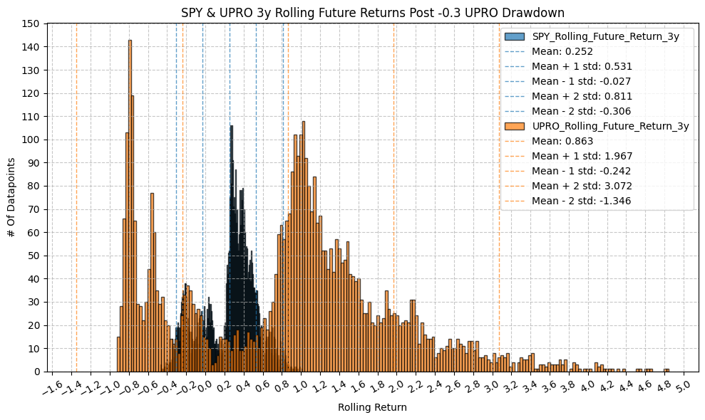
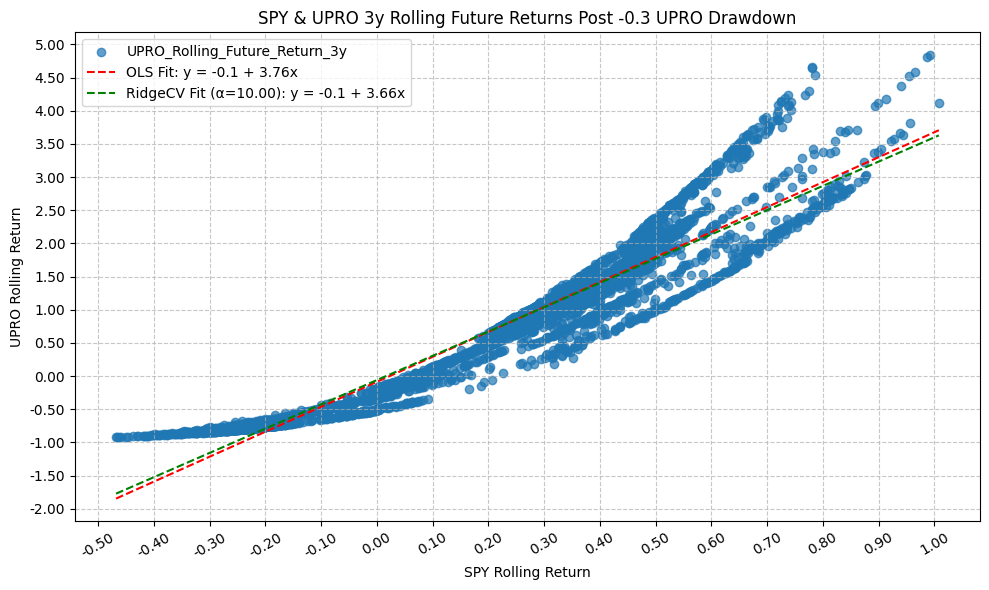
OLS Regression Results
=========================================================================================
Dep. Variable: UPRO_Rolling_Future_Return_3y R-squared: 0.904
Model: OLS Adj. R-squared: 0.904
Method: Least Squares F-statistic: 4.267e+04
Date: Mon, 23 Mar 2026 Prob (F-statistic): 0.00
Time: 22:03:25 Log-Likelihood: -1584.5
No. Observations: 4550 AIC: 3173.
Df Residuals: 4548 BIC: 3186.
Df Model: 1
Covariance Type: nonrobust
================================================================================================
coef std err t P>|t| [0.025 0.975]
------------------------------------------------------------------------------------------------
const -0.0863 0.007 -12.589 0.000 -0.100 -0.073
SPY_Rolling_Future_Return_3y 3.7615 0.018 206.575 0.000 3.726 3.797
==============================================================================
Omnibus: 690.118 Durbin-Watson: 0.019
Prob(Omnibus): 0.000 Jarque-Bera (JB): 1788.637
Skew: 0.837 Prob(JB): 0.00
Kurtosis: 5.576 Cond. No. 3.83
==============================================================================
Notes:
[1] Standard Errors assume that the covariance matrix of the errors is correctly specified.
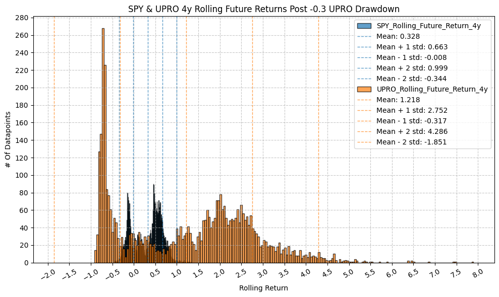
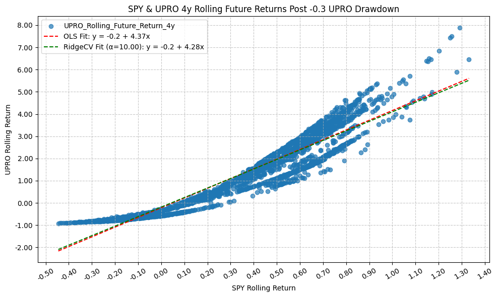
OLS Regression Results
=========================================================================================
Dep. Variable: UPRO_Rolling_Future_Return_4y R-squared: 0.916
Model: OLS Adj. R-squared: 0.915
Method: Least Squares F-statistic: 4.683e+04
Date: Mon, 23 Mar 2026 Prob (F-statistic): 0.00
Time: 22:03:26 Log-Likelihood: -2643.5
No. Observations: 4324 AIC: 5291.
Df Residuals: 4322 BIC: 5304.
Df Model: 1
Covariance Type: nonrobust
================================================================================================
coef std err t P>|t| [0.025 0.975]
------------------------------------------------------------------------------------------------
const -0.2147 0.009 -22.658 0.000 -0.233 -0.196
SPY_Rolling_Future_Return_4y 4.3728 0.020 216.406 0.000 4.333 4.412
==============================================================================
Omnibus: 116.085 Durbin-Watson: 0.023
Prob(Omnibus): 0.000 Jarque-Bera (JB): 243.926
Skew: -0.150 Prob(JB): 1.08e-53
Kurtosis: 4.124 Cond. No. 3.33
==============================================================================
Notes:
[1] Standard Errors assume that the covariance matrix of the errors is correctly specified.
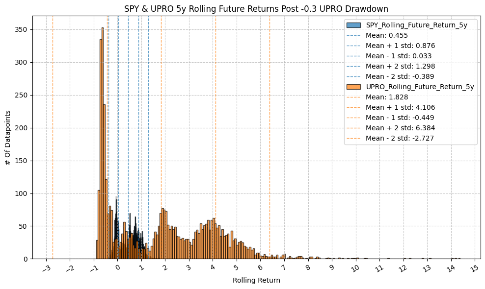
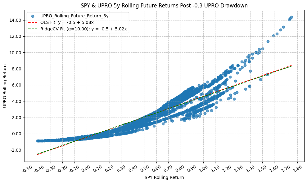
OLS Regression Results
=========================================================================================
Dep. Variable: UPRO_Rolling_Future_Return_5y R-squared: 0.887
Model: OLS Adj. R-squared: 0.887
Method: Least Squares F-statistic: 3.391e+04
Date: Mon, 23 Mar 2026 Prob (F-statistic): 0.00
Time: 22:03:28 Log-Likelihood: -4969.8
No. Observations: 4317 AIC: 9944.
Df Residuals: 4315 BIC: 9956.
Df Model: 1
Covariance Type: nonrobust
================================================================================================
coef std err t P>|t| [0.025 0.975]
------------------------------------------------------------------------------------------------
const -0.4824 0.017 -28.173 0.000 -0.516 -0.449
SPY_Rolling_Future_Return_5y 5.0840 0.028 184.148 0.000 5.030 5.138
==============================================================================
Omnibus: 712.609 Durbin-Watson: 0.017
Prob(Omnibus): 0.000 Jarque-Bera (JB): 3461.216
Skew: 0.712 Prob(JB): 0.00
Kurtosis: 7.149 Cond. No. 2.94
==============================================================================
Notes:
[1] Standard Errors assume that the covariance matrix of the errors is correctly specified.

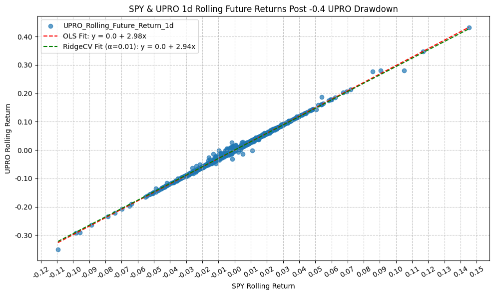
OLS Regression Results
=========================================================================================
Dep. Variable: UPRO_Rolling_Future_Return_1d R-squared: 0.997
Model: OLS Adj. R-squared: 0.997
Method: Least Squares F-statistic: 1.487e+06
Date: Mon, 23 Mar 2026 Prob (F-statistic): 0.00
Time: 22:03:30 Log-Likelihood: 21081.
No. Observations: 4464 AIC: -4.216e+04
Df Residuals: 4462 BIC: -4.214e+04
Df Model: 1
Covariance Type: nonrobust
================================================================================================
coef std err t P>|t| [0.025 0.975]
------------------------------------------------------------------------------------------------
const 4.4e-05 3.22e-05 1.365 0.172 -1.92e-05 0.000
SPY_Rolling_Future_Return_1d 2.9791 0.002 1219.596 0.000 2.974 2.984
==============================================================================
Omnibus: 2686.462 Durbin-Watson: 2.619
Prob(Omnibus): 0.000 Jarque-Bera (JB): 1502620.805
Skew: 1.531 Prob(JB): 0.00
Kurtosis: 92.829 Cond. No. 75.8
==============================================================================
Notes:
[1] Standard Errors assume that the covariance matrix of the errors is correctly specified.


OLS Regression Results
=========================================================================================
Dep. Variable: UPRO_Rolling_Future_Return_1w R-squared: 0.993
Model: OLS Adj. R-squared: 0.993
Method: Least Squares F-statistic: 6.179e+05
Date: Mon, 23 Mar 2026 Prob (F-statistic): 0.00
Time: 22:03:32 Log-Likelihood: 16080.
No. Observations: 4464 AIC: -3.216e+04
Df Residuals: 4462 BIC: -3.214e+04
Df Model: 1
Covariance Type: nonrobust
================================================================================================
coef std err t P>|t| [0.025 0.975]
------------------------------------------------------------------------------------------------
const -0.0002 9.9e-05 -1.776 0.076 -0.000 1.83e-05
SPY_Rolling_Future_Return_1w 2.9716 0.004 786.087 0.000 2.964 2.979
==============================================================================
Omnibus: 1977.646 Durbin-Watson: 0.971
Prob(Omnibus): 0.000 Jarque-Bera (JB): 519446.713
Skew: -0.905 Prob(JB): 0.00
Kurtosis: 55.815 Cond. No. 38.3
==============================================================================
Notes:
[1] Standard Errors assume that the covariance matrix of the errors is correctly specified.
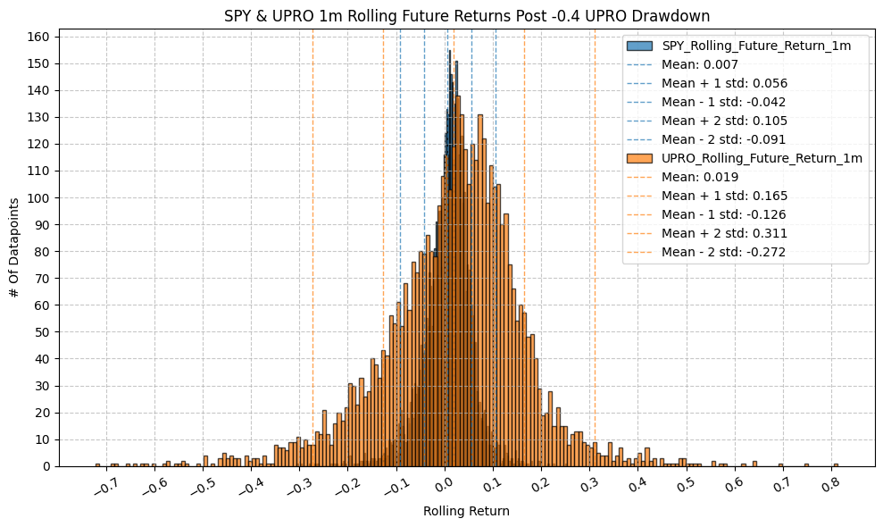

OLS Regression Results
=========================================================================================
Dep. Variable: UPRO_Rolling_Future_Return_1m R-squared: 0.986
Model: OLS Adj. R-squared: 0.986
Method: Least Squares F-statistic: 3.225e+05
Date: Mon, 23 Mar 2026 Prob (F-statistic): 0.00
Time: 22:03:33 Log-Likelihood: 11851.
No. Observations: 4464 AIC: -2.370e+04
Df Residuals: 4462 BIC: -2.368e+04
Df Model: 1
Covariance Type: nonrobust
================================================================================================
coef std err t P>|t| [0.025 0.975]
------------------------------------------------------------------------------------------------
const -0.0009 0.000 -3.419 0.001 -0.001 -0.000
SPY_Rolling_Future_Return_1m 2.9519 0.005 567.906 0.000 2.942 2.962
==============================================================================
Omnibus: 2549.897 Durbin-Watson: 0.358
Prob(Omnibus): 0.000 Jarque-Bera (JB): 256138.956
Skew: -1.810 Prob(JB): 0.00
Kurtosis: 39.932 Cond. No. 20.4
==============================================================================
Notes:
[1] Standard Errors assume that the covariance matrix of the errors is correctly specified.
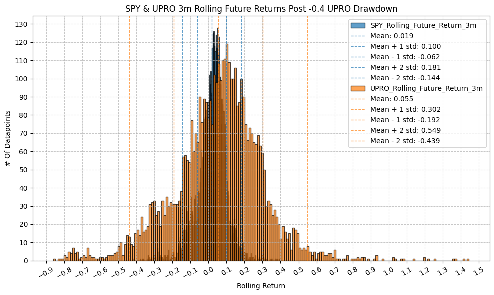

OLS Regression Results
=========================================================================================
Dep. Variable: UPRO_Rolling_Future_Return_3m R-squared: 0.978
Model: OLS Adj. R-squared: 0.978
Method: Least Squares F-statistic: 2.007e+05
Date: Mon, 23 Mar 2026 Prob (F-statistic): 0.00
Time: 22:03:35 Log-Likelihood: 8451.7
No. Observations: 4464 AIC: -1.690e+04
Df Residuals: 4462 BIC: -1.689e+04
Df Model: 1
Covariance Type: nonrobust
================================================================================================
coef std err t P>|t| [0.025 0.975]
------------------------------------------------------------------------------------------------
const -0.0018 0.001 -3.144 0.002 -0.003 -0.001
SPY_Rolling_Future_Return_3m 3.0074 0.007 448.025 0.000 2.994 3.021
==============================================================================
Omnibus: 1648.657 Durbin-Watson: 0.182
Prob(Omnibus): 0.000 Jarque-Bera (JB): 57080.700
Skew: 1.101 Prob(JB): 0.00
Kurtosis: 20.379 Cond. No. 12.3
==============================================================================
Notes:
[1] Standard Errors assume that the covariance matrix of the errors is correctly specified.
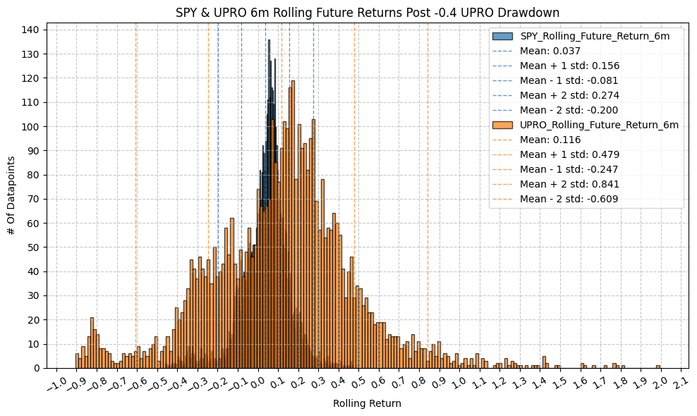

OLS Regression Results
=========================================================================================
Dep. Variable: UPRO_Rolling_Future_Return_6m R-squared: 0.959
Model: OLS Adj. R-squared: 0.959
Method: Least Squares F-statistic: 1.039e+05
Date: Mon, 23 Mar 2026 Prob (F-statistic): 0.00
Time: 22:03:37 Log-Likelihood: 5314.6
No. Observations: 4464 AIC: -1.063e+04
Df Residuals: 4462 BIC: -1.061e+04
Df Model: 1
Covariance Type: nonrobust
================================================================================================
coef std err t P>|t| [0.025 0.975]
------------------------------------------------------------------------------------------------
const 0.0040 0.001 3.496 0.000 0.002 0.006
SPY_Rolling_Future_Return_6m 2.9973 0.009 322.292 0.000 2.979 3.015
==============================================================================
Omnibus: 1611.711 Durbin-Watson: 0.081
Prob(Omnibus): 0.000 Jarque-Bera (JB): 13011.898
Skew: 1.500 Prob(JB): 0.00
Kurtosis: 10.808 Cond. No. 8.46
==============================================================================
Notes:
[1] Standard Errors assume that the covariance matrix of the errors is correctly specified.

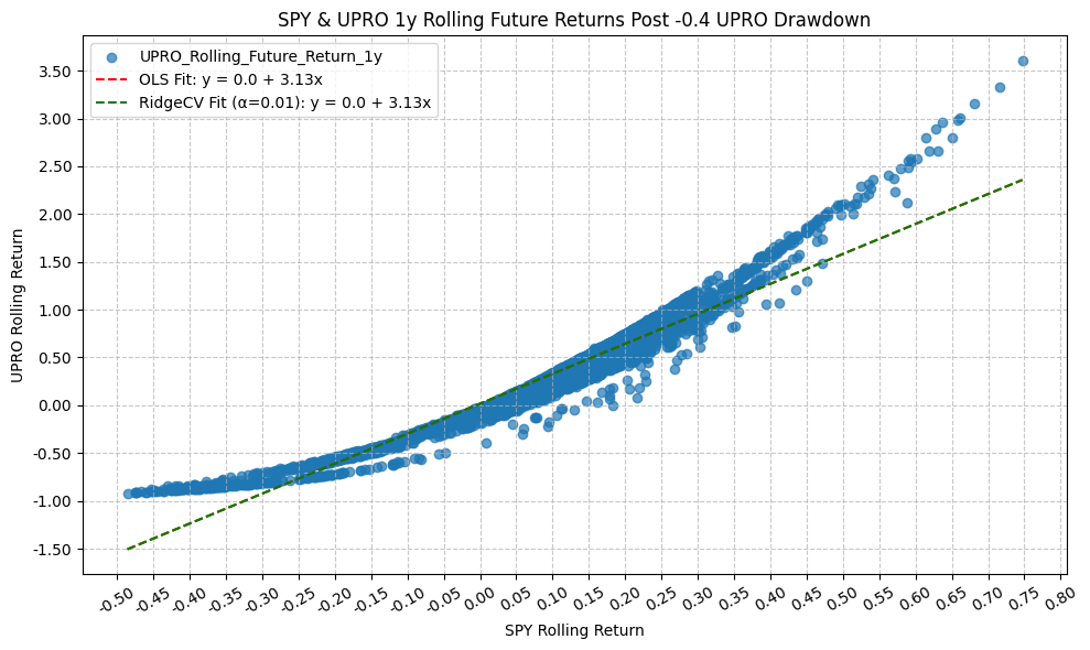
OLS Regression Results
=========================================================================================
Dep. Variable: UPRO_Rolling_Future_Return_1y R-squared: 0.936
Model: OLS Adj. R-squared: 0.936
Method: Least Squares F-statistic: 6.492e+04
Date: Mon, 23 Mar 2026 Prob (F-statistic): 0.00
Time: 22:03:38 Log-Likelihood: 2334.8
No. Observations: 4456 AIC: -4666.
Df Residuals: 4454 BIC: -4653.
Df Model: 1
Covariance Type: nonrobust
================================================================================================
coef std err t P>|t| [0.025 0.975]
------------------------------------------------------------------------------------------------
const 0.0162 0.002 6.864 0.000 0.012 0.021
SPY_Rolling_Future_Return_1y 3.1340 0.012 254.788 0.000 3.110 3.158
==============================================================================
Omnibus: 1684.730 Durbin-Watson: 0.054
Prob(Omnibus): 0.000 Jarque-Bera (JB): 11774.002
Skew: 1.634 Prob(JB): 0.00
Kurtosis: 10.262 Cond. No. 5.77
==============================================================================
Notes:
[1] Standard Errors assume that the covariance matrix of the errors is correctly specified.

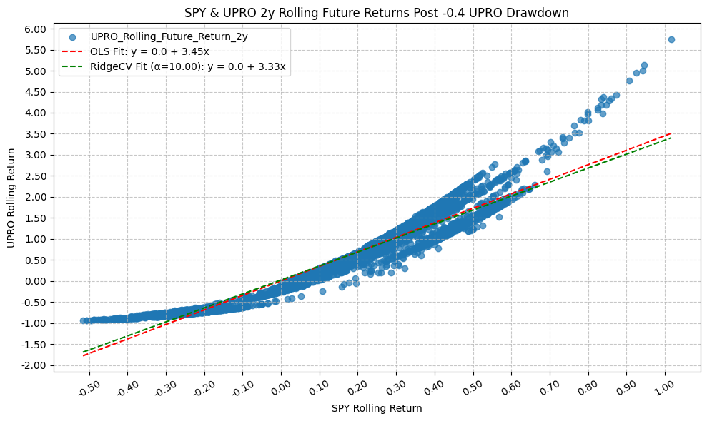
OLS Regression Results
=========================================================================================
Dep. Variable: UPRO_Rolling_Future_Return_2y R-squared: 0.907
Model: OLS Adj. R-squared: 0.907
Method: Least Squares F-statistic: 4.353e+04
Date: Mon, 23 Mar 2026 Prob (F-statistic): 0.00
Time: 22:03:40 Log-Likelihood: -457.01
No. Observations: 4456 AIC: 918.0
Df Residuals: 4454 BIC: 930.8
Df Model: 1
Covariance Type: nonrobust
================================================================================================
coef std err t P>|t| [0.025 0.975]
------------------------------------------------------------------------------------------------
const 0.0011 0.005 0.224 0.823 -0.009 0.011
SPY_Rolling_Future_Return_2y 3.4516 0.017 208.650 0.000 3.419 3.484
==============================================================================
Omnibus: 1243.396 Durbin-Watson: 0.033
Prob(Omnibus): 0.000 Jarque-Bera (JB): 4602.198
Skew: 1.354 Prob(JB): 0.00
Kurtosis: 7.178 Cond. No. 4.25
==============================================================================
Notes:
[1] Standard Errors assume that the covariance matrix of the errors is correctly specified.
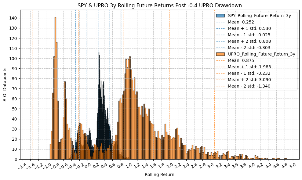
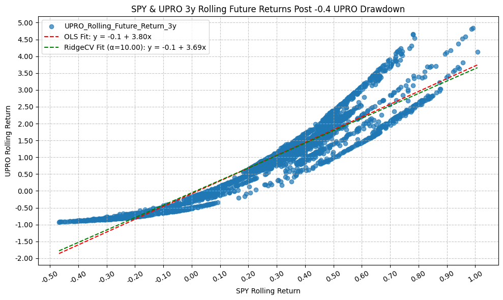
OLS Regression Results
=========================================================================================
Dep. Variable: UPRO_Rolling_Future_Return_3y R-squared: 0.907
Model: OLS Adj. R-squared: 0.907
Method: Least Squares F-statistic: 4.211e+04
Date: Mon, 23 Mar 2026 Prob (F-statistic): 0.00
Time: 22:03:42 Log-Likelihood: -1446.7
No. Observations: 4328 AIC: 2897.
Df Residuals: 4326 BIC: 2910.
Df Model: 1
Covariance Type: nonrobust
================================================================================================
coef std err t P>|t| [0.025 0.975]
------------------------------------------------------------------------------------------------
const -0.0835 0.007 -12.022 0.000 -0.097 -0.070
SPY_Rolling_Future_Return_3y 3.7973 0.019 205.205 0.000 3.761 3.834
==============================================================================
Omnibus: 704.595 Durbin-Watson: 0.022
Prob(Omnibus): 0.000 Jarque-Bera (JB): 1810.678
Skew: 0.895 Prob(JB): 0.00
Kurtosis: 5.615 Cond. No. 3.85
==============================================================================
Notes:
[1] Standard Errors assume that the covariance matrix of the errors is correctly specified.
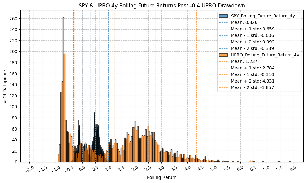
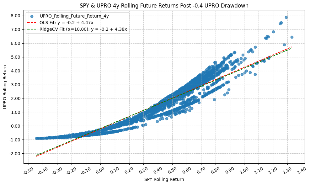
OLS Regression Results
=========================================================================================
Dep. Variable: UPRO_Rolling_Future_Return_4y R-squared: 0.926
Model: OLS Adj. R-squared: 0.926
Method: Least Squares F-statistic: 5.187e+04
Date: Mon, 23 Mar 2026 Prob (F-statistic): 0.00
Time: 22:03:43 Log-Likelihood: -2273.5
No. Observations: 4126 AIC: 4551.
Df Residuals: 4124 BIC: 4564.
Df Model: 1
Covariance Type: nonrobust
================================================================================================
coef std err t P>|t| [0.025 0.975]
------------------------------------------------------------------------------------------------
const -0.2232 0.009 -24.382 0.000 -0.241 -0.205
SPY_Rolling_Future_Return_4y 4.4750 0.020 227.749 0.000 4.436 4.513
==============================================================================
Omnibus: 119.459 Durbin-Watson: 0.024
Prob(Omnibus): 0.000 Jarque-Bera (JB): 294.579
Skew: -0.074 Prob(JB): 1.08e-64
Kurtosis: 4.301 Cond. No. 3.36
==============================================================================
Notes:
[1] Standard Errors assume that the covariance matrix of the errors is correctly specified.
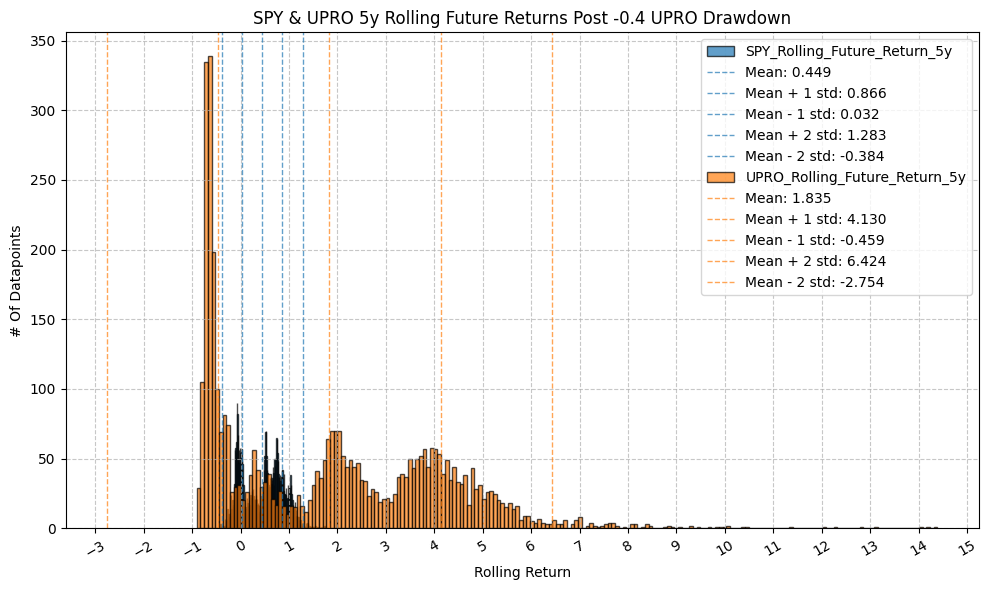

OLS Regression Results
=========================================================================================
Dep. Variable: UPRO_Rolling_Future_Return_5y R-squared: 0.896
Model: OLS Adj. R-squared: 0.896
Method: Least Squares F-statistic: 3.555e+04
Date: Mon, 23 Mar 2026 Prob (F-statistic): 0.00
Time: 22:03:45 Log-Likelihood: -4610.5
No. Observations: 4126 AIC: 9225.
Df Residuals: 4124 BIC: 9238.
Df Model: 1
Covariance Type: nonrobust
================================================================================================
coef std err t P>|t| [0.025 0.975]
------------------------------------------------------------------------------------------------
const -0.5058 0.017 -29.864 0.000 -0.539 -0.473
SPY_Rolling_Future_Return_5y 5.2121 0.028 188.535 0.000 5.158 5.266
==============================================================================
Omnibus: 688.391 Durbin-Watson: 0.019
Prob(Omnibus): 0.000 Jarque-Bera (JB): 3304.496
Skew: 0.724 Prob(JB): 0.00
Kurtosis: 7.138 Cond. No. 2.96
==============================================================================
Notes:
[1] Standard Errors assume that the covariance matrix of the errors is correctly specified.

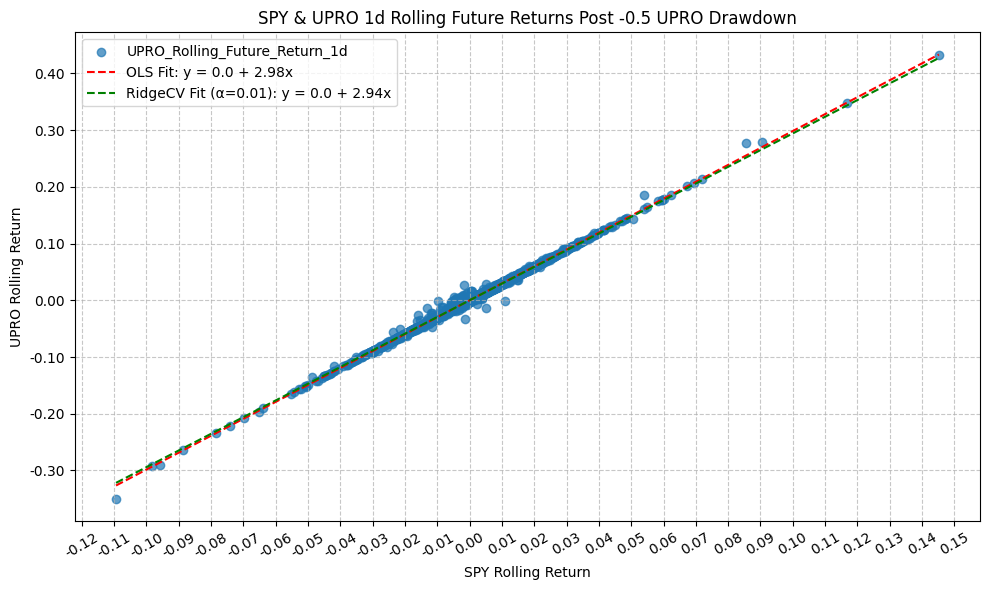
OLS Regression Results
=========================================================================================
Dep. Variable: UPRO_Rolling_Future_Return_1d R-squared: 0.997
Model: OLS Adj. R-squared: 0.997
Method: Least Squares F-statistic: 1.337e+06
Date: Mon, 23 Mar 2026 Prob (F-statistic): 0.00
Time: 22:03:47 Log-Likelihood: 18275.
No. Observations: 3869 AIC: -3.655e+04
Df Residuals: 3867 BIC: -3.653e+04
Df Model: 1
Covariance Type: nonrobust
================================================================================================
coef std err t P>|t| [0.025 0.975]
------------------------------------------------------------------------------------------------
const 5.793e-05 3.46e-05 1.675 0.094 -9.88e-06 0.000
SPY_Rolling_Future_Return_1d 2.9842 0.003 1156.072 0.000 2.979 2.989
==============================================================================
Omnibus: 2831.178 Durbin-Watson: 2.689
Prob(Omnibus): 0.000 Jarque-Bera (JB): 1196713.827
Skew: 2.308 Prob(JB): 0.00
Kurtosis: 89.035 Cond. No. 74.7
==============================================================================
Notes:
[1] Standard Errors assume that the covariance matrix of the errors is correctly specified.

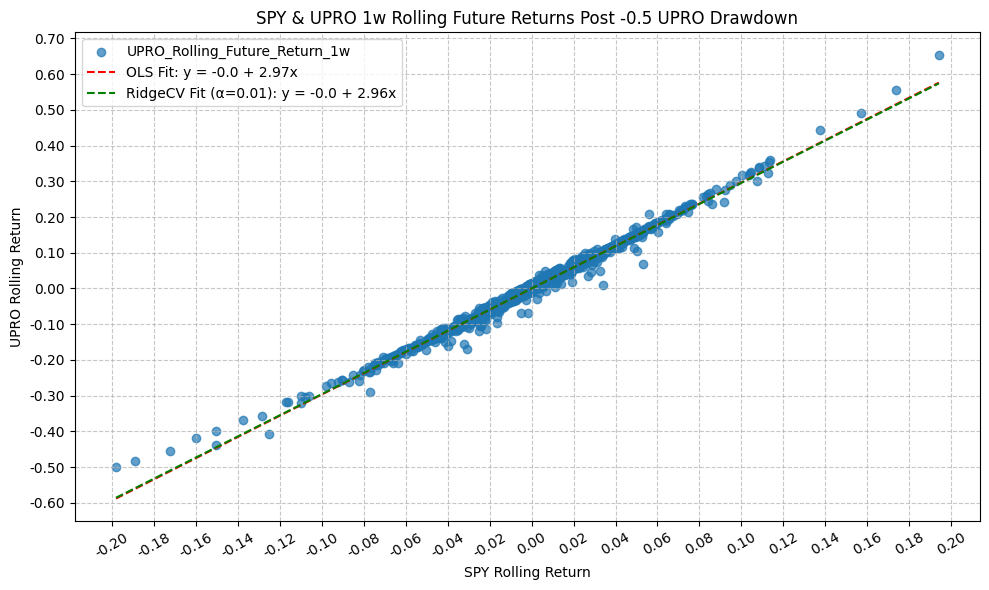
OLS Regression Results
=========================================================================================
Dep. Variable: UPRO_Rolling_Future_Return_1w R-squared: 0.993
Model: OLS Adj. R-squared: 0.993
Method: Least Squares F-statistic: 5.120e+05
Date: Mon, 23 Mar 2026 Prob (F-statistic): 0.00
Time: 22:03:49 Log-Likelihood: 13820.
No. Observations: 3869 AIC: -2.764e+04
Df Residuals: 3867 BIC: -2.762e+04
Df Model: 1
Covariance Type: nonrobust
================================================================================================
coef std err t P>|t| [0.025 0.975]
------------------------------------------------------------------------------------------------
const -0.0001 0.000 -0.991 0.322 -0.000 0.000
SPY_Rolling_Future_Return_1w 2.9702 0.004 715.546 0.000 2.962 2.978
==============================================================================
Omnibus: 1718.530 Durbin-Watson: 1.003
Prob(Omnibus): 0.000 Jarque-Bera (JB): 451630.478
Skew: -0.906 Prob(JB): 0.00
Kurtosis: 55.899 Cond. No. 38.0
==============================================================================
Notes:
[1] Standard Errors assume that the covariance matrix of the errors is correctly specified.
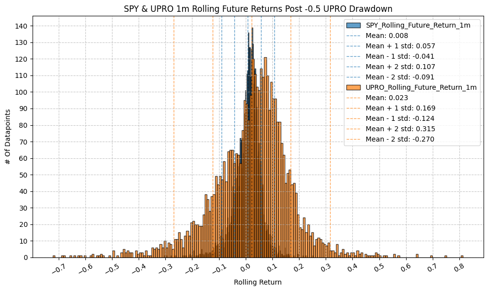
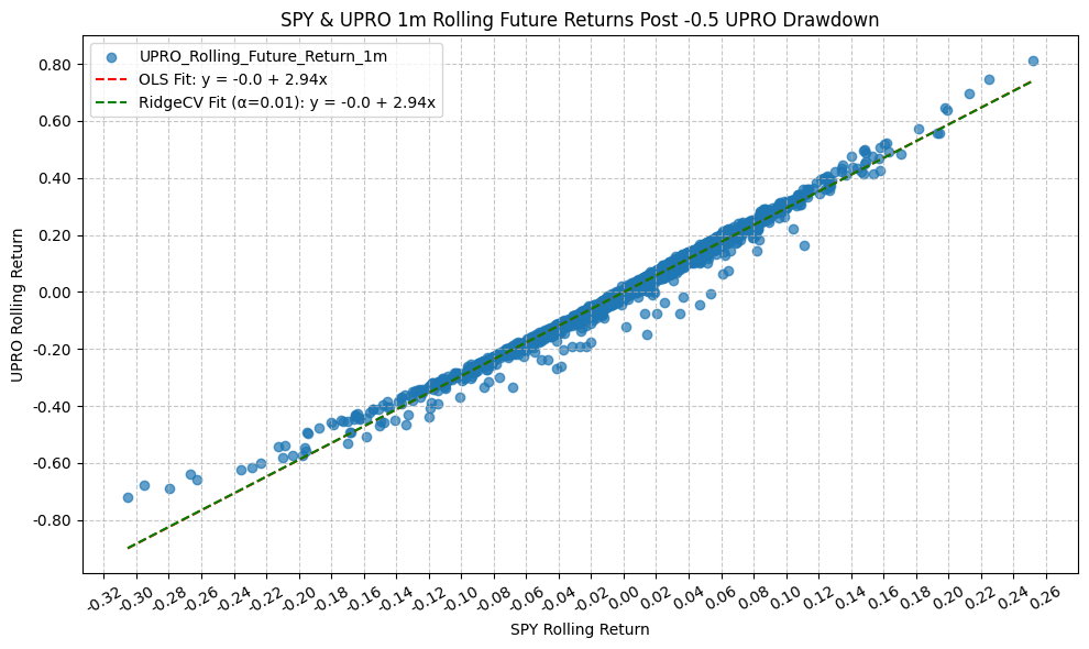
OLS Regression Results
=========================================================================================
Dep. Variable: UPRO_Rolling_Future_Return_1m R-squared: 0.986
Model: OLS Adj. R-squared: 0.986
Method: Least Squares F-statistic: 2.737e+05
Date: Mon, 23 Mar 2026 Prob (F-statistic): 0.00
Time: 22:03:51 Log-Likelihood: 10213.
No. Observations: 3869 AIC: -2.042e+04
Df Residuals: 3867 BIC: -2.041e+04
Df Model: 1
Covariance Type: nonrobust
================================================================================================
coef std err t P>|t| [0.025 0.975]
------------------------------------------------------------------------------------------------
const -0.0008 0.000 -2.729 0.006 -0.001 -0.000
SPY_Rolling_Future_Return_1m 2.9438 0.006 523.149 0.000 2.933 2.955
==============================================================================
Omnibus: 2104.983 Durbin-Watson: 0.385
Prob(Omnibus): 0.000 Jarque-Bera (JB): 199121.381
Skew: -1.679 Prob(JB): 0.00
Kurtosis: 37.984 Cond. No. 20.3
==============================================================================
Notes:
[1] Standard Errors assume that the covariance matrix of the errors is correctly specified.
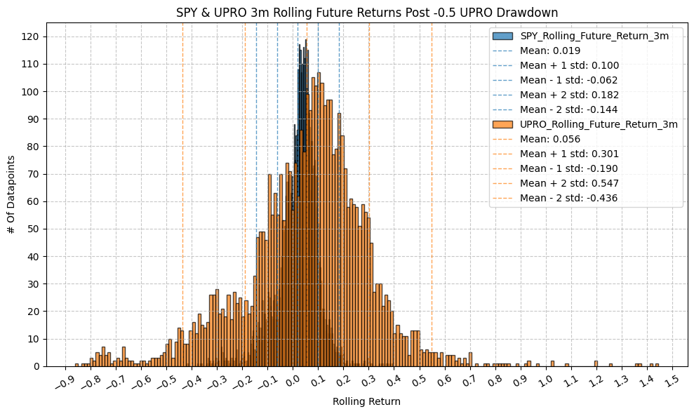

OLS Regression Results
=========================================================================================
Dep. Variable: UPRO_Rolling_Future_Return_3m R-squared: 0.978
Model: OLS Adj. R-squared: 0.978
Method: Least Squares F-statistic: 1.700e+05
Date: Mon, 23 Mar 2026 Prob (F-statistic): 0.00
Time: 22:03:52 Log-Likelihood: 7302.1
No. Observations: 3869 AIC: -1.460e+04
Df Residuals: 3867 BIC: -1.459e+04
Df Model: 1
Covariance Type: nonrobust
================================================================================================
coef std err t P>|t| [0.025 0.975]
------------------------------------------------------------------------------------------------
const -0.0011 0.001 -1.895 0.058 -0.002 3.98e-05
SPY_Rolling_Future_Return_3m 2.9839 0.007 412.319 0.000 2.970 2.998
==============================================================================
Omnibus: 1374.050 Durbin-Watson: 0.193
Prob(Omnibus): 0.000 Jarque-Bera (JB): 42996.583
Skew: 1.059 Prob(JB): 0.00
Kurtosis: 19.194 Cond. No. 12.3
==============================================================================
Notes:
[1] Standard Errors assume that the covariance matrix of the errors is correctly specified.
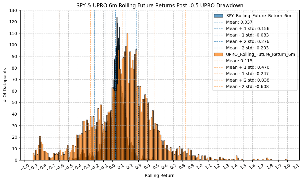
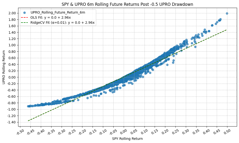
OLS Regression Results
=========================================================================================
Dep. Variable: UPRO_Rolling_Future_Return_6m R-squared: 0.957
Model: OLS Adj. R-squared: 0.957
Method: Least Squares F-statistic: 8.586e+04
Date: Mon, 23 Mar 2026 Prob (F-statistic): 0.00
Time: 22:03:54 Log-Likelihood: 4529.2
No. Observations: 3869 AIC: -9054.
Df Residuals: 3867 BIC: -9042.
Df Model: 1
Covariance Type: nonrobust
================================================================================================
coef std err t P>|t| [0.025 0.975]
------------------------------------------------------------------------------------------------
const 0.0067 0.001 5.303 0.000 0.004 0.009
SPY_Rolling_Future_Return_6m 2.9568 0.010 293.014 0.000 2.937 2.977
==============================================================================
Omnibus: 1291.522 Durbin-Watson: 0.081
Prob(Omnibus): 0.000 Jarque-Bera (JB): 9377.484
Skew: 1.396 Prob(JB): 0.00
Kurtosis: 10.098 Cond. No. 8.37
==============================================================================
Notes:
[1] Standard Errors assume that the covariance matrix of the errors is correctly specified.


OLS Regression Results
=========================================================================================
Dep. Variable: UPRO_Rolling_Future_Return_1y R-squared: 0.933
Model: OLS Adj. R-squared: 0.933
Method: Least Squares F-statistic: 5.405e+04
Date: Mon, 23 Mar 2026 Prob (F-statistic): 0.00
Time: 22:03:56 Log-Likelihood: 1956.3
No. Observations: 3869 AIC: -3909.
Df Residuals: 3867 BIC: -3896.
Df Model: 1
Covariance Type: nonrobust
================================================================================================
coef std err t P>|t| [0.025 0.975]
------------------------------------------------------------------------------------------------
const 0.0175 0.003 6.793 0.000 0.012 0.023
SPY_Rolling_Future_Return_1y 3.1290 0.013 232.490 0.000 3.103 3.155
==============================================================================
Omnibus: 1513.598 Durbin-Watson: 0.057
Prob(Omnibus): 0.000 Jarque-Bera (JB): 11118.231
Skew: 1.681 Prob(JB): 0.00
Kurtosis: 10.594 Cond. No. 5.77
==============================================================================
Notes:
[1] Standard Errors assume that the covariance matrix of the errors is correctly specified.
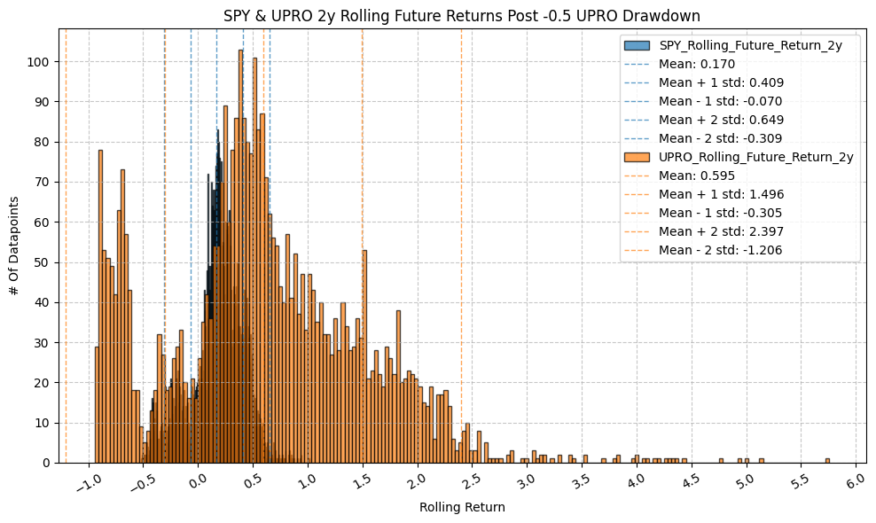
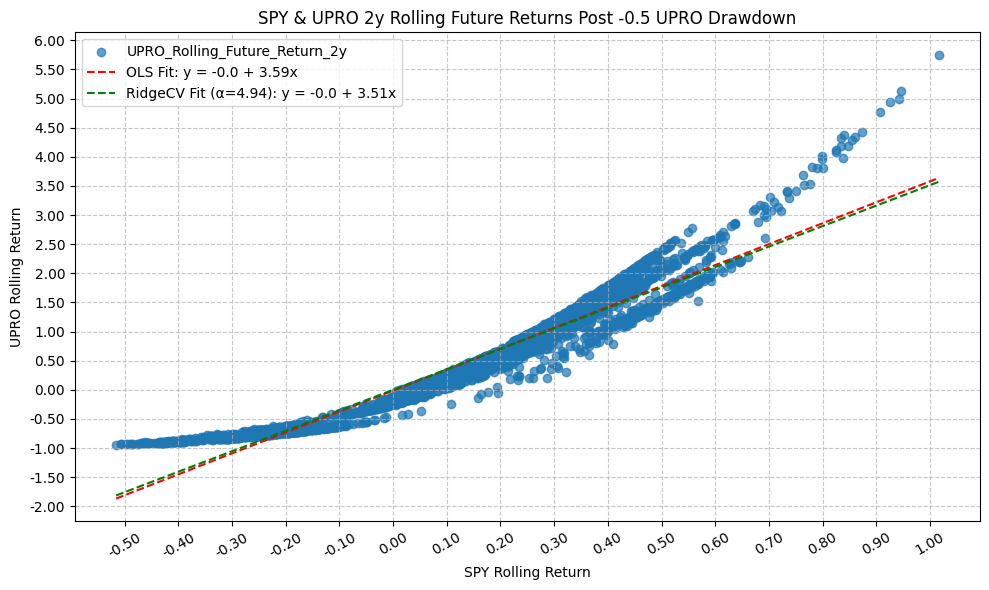
OLS Regression Results
=========================================================================================
Dep. Variable: UPRO_Rolling_Future_Return_2y R-squared: 0.912
Model: OLS Adj. R-squared: 0.912
Method: Least Squares F-statistic: 4.020e+04
Date: Mon, 23 Mar 2026 Prob (F-statistic): 0.00
Time: 22:03:57 Log-Likelihood: -378.23
No. Observations: 3869 AIC: 760.5
Df Residuals: 3867 BIC: 773.0
Df Model: 1
Covariance Type: nonrobust
================================================================================================
coef std err t P>|t| [0.025 0.975]
------------------------------------------------------------------------------------------------
const -0.0141 0.005 -2.682 0.007 -0.024 -0.004
SPY_Rolling_Future_Return_2y 3.5919 0.018 200.490 0.000 3.557 3.627
==============================================================================
Omnibus: 1083.389 Durbin-Watson: 0.036
Prob(Omnibus): 0.000 Jarque-Bera (JB): 3625.480
Skew: 1.395 Prob(JB): 0.00
Kurtosis: 6.835 Cond. No. 4.30
==============================================================================
Notes:
[1] Standard Errors assume that the covariance matrix of the errors is correctly specified.
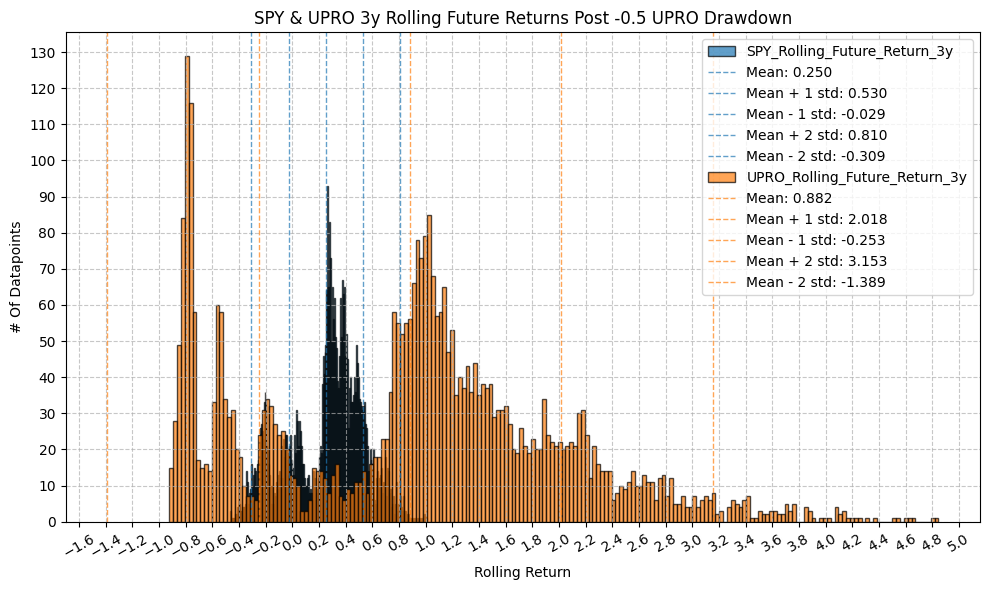
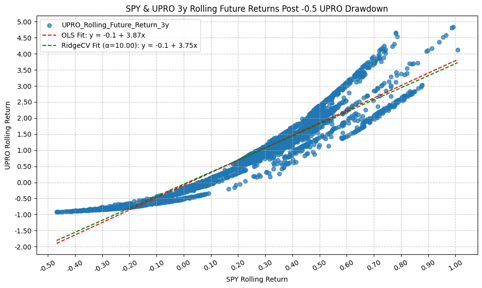
OLS Regression Results
=========================================================================================
Dep. Variable: UPRO_Rolling_Future_Return_3y R-squared: 0.911
Model: OLS Adj. R-squared: 0.911
Method: Least Squares F-statistic: 3.905e+04
Date: Mon, 23 Mar 2026 Prob (F-statistic): 0.00
Time: 22:03:59 Log-Likelihood: -1297.7
No. Observations: 3835 AIC: 2599.
Df Residuals: 3833 BIC: 2612.
Df Model: 1
Covariance Type: nonrobust
================================================================================================
coef std err t P>|t| [0.025 0.975]
------------------------------------------------------------------------------------------------
const -0.0881 0.007 -11.975 0.000 -0.103 -0.074
SPY_Rolling_Future_Return_3y 3.8745 0.020 197.618 0.000 3.836 3.913
==============================================================================
Omnibus: 633.347 Durbin-Watson: 0.022
Prob(Omnibus): 0.000 Jarque-Bera (JB): 1404.095
Skew: 0.957 Prob(JB): 1.27e-305
Kurtosis: 5.264 Cond. No. 3.82
==============================================================================
Notes:
[1] Standard Errors assume that the covariance matrix of the errors is correctly specified.
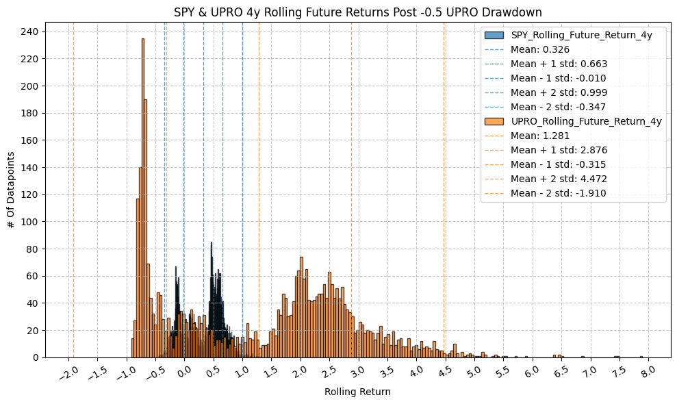
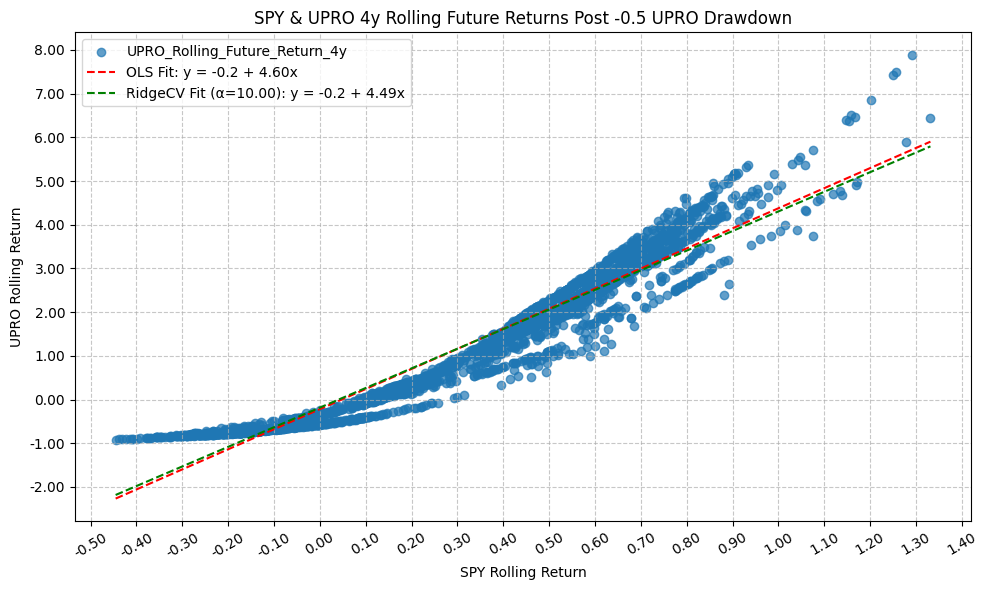
OLS Regression Results
=========================================================================================
Dep. Variable: UPRO_Rolling_Future_Return_4y R-squared: 0.940
Model: OLS Adj. R-squared: 0.940
Method: Least Squares F-statistic: 5.808e+04
Date: Mon, 23 Mar 2026 Prob (F-statistic): 0.00
Time: 22:04:01 Log-Likelihood: -1763.7
No. Observations: 3694 AIC: 3531.
Df Residuals: 3692 BIC: 3544.
Df Model: 1
Covariance Type: nonrobust
================================================================================================
coef std err t P>|t| [0.025 0.975]
------------------------------------------------------------------------------------------------
const -0.2198 0.009 -24.572 0.000 -0.237 -0.202
SPY_Rolling_Future_Return_4y 4.5977 0.019 240.993 0.000 4.560 4.635
==============================================================================
Omnibus: 140.743 Durbin-Watson: 0.030
Prob(Omnibus): 0.000 Jarque-Bera (JB): 414.327
Skew: 0.067 Prob(JB): 1.07e-90
Kurtosis: 4.635 Cond. No. 3.32
==============================================================================
Notes:
[1] Standard Errors assume that the covariance matrix of the errors is correctly specified.
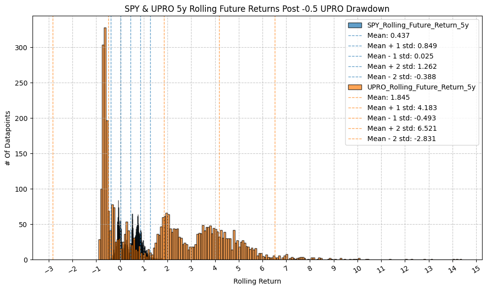
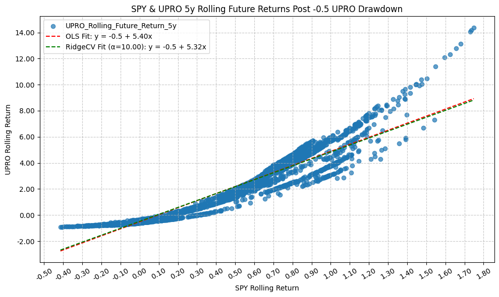
OLS Regression Results
=========================================================================================
Dep. Variable: UPRO_Rolling_Future_Return_5y R-squared: 0.907
Model: OLS Adj. R-squared: 0.907
Method: Least Squares F-statistic: 3.596e+04
Date: Mon, 23 Mar 2026 Prob (F-statistic): 0.00
Time: 22:04:02 Log-Likelihood: -3993.5
No. Observations: 3694 AIC: 7991.
Df Residuals: 3692 BIC: 8003.
Df Model: 1
Covariance Type: nonrobust
================================================================================================
coef std err t P>|t| [0.025 0.975]
------------------------------------------------------------------------------------------------
const -0.5138 0.017 -30.038 0.000 -0.547 -0.480
SPY_Rolling_Future_Return_5y 5.3997 0.028 189.643 0.000 5.344 5.456
==============================================================================
Omnibus: 550.645 Durbin-Watson: 0.022
Prob(Omnibus): 0.000 Jarque-Bera (JB): 2880.308
Skew: 0.608 Prob(JB): 0.00
Kurtosis: 7.151 Cond. No. 2.96
==============================================================================
Notes:
[1] Standard Errors assume that the covariance matrix of the errors is correctly specified.

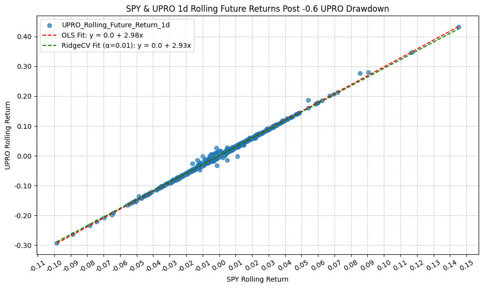
OLS Regression Results
=========================================================================================
Dep. Variable: UPRO_Rolling_Future_Return_1d R-squared: 0.997
Model: OLS Adj. R-squared: 0.997
Method: Least Squares F-statistic: 1.059e+06
Date: Mon, 23 Mar 2026 Prob (F-statistic): 0.00
Time: 22:04:04 Log-Likelihood: 14432.
No. Observations: 3070 AIC: -2.886e+04
Df Residuals: 3068 BIC: -2.885e+04
Df Model: 1
Covariance Type: nonrobust
================================================================================================
coef std err t P>|t| [0.025 0.975]
------------------------------------------------------------------------------------------------
const 7.426e-05 3.97e-05 1.869 0.062 -3.64e-06 0.000
SPY_Rolling_Future_Return_1d 2.9824 0.003 1028.858 0.000 2.977 2.988
==============================================================================
Omnibus: 2273.415 Durbin-Watson: 2.537
Prob(Omnibus): 0.000 Jarque-Bera (JB): 1052816.390
Skew: 2.319 Prob(JB): 0.00
Kurtosis: 93.603 Cond. No. 73.0
==============================================================================
Notes:
[1] Standard Errors assume that the covariance matrix of the errors is correctly specified.


OLS Regression Results
=========================================================================================
Dep. Variable: UPRO_Rolling_Future_Return_1w R-squared: 0.992
Model: OLS Adj. R-squared: 0.992
Method: Least Squares F-statistic: 3.762e+05
Date: Mon, 23 Mar 2026 Prob (F-statistic): 0.00
Time: 22:04:06 Log-Likelihood: 10750.
No. Observations: 3070 AIC: -2.150e+04
Df Residuals: 3068 BIC: -2.148e+04
Df Model: 1
Covariance Type: nonrobust
================================================================================================
coef std err t P>|t| [0.025 0.975]
------------------------------------------------------------------------------------------------
const -0.0001 0.000 -1.041 0.298 -0.000 0.000
SPY_Rolling_Future_Return_1w 2.9677 0.005 613.333 0.000 2.958 2.977
==============================================================================
Omnibus: 1399.487 Durbin-Watson: 1.060
Prob(Omnibus): 0.000 Jarque-Bera (JB): 313356.086
Skew: -0.996 Prob(JB): 0.00
Kurtosis: 52.454 Cond. No. 36.7
==============================================================================
Notes:
[1] Standard Errors assume that the covariance matrix of the errors is correctly specified.
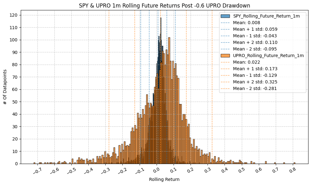
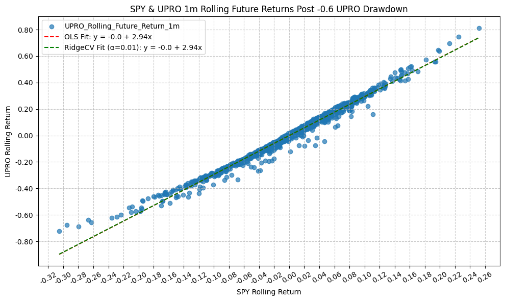
OLS Regression Results
=========================================================================================
Dep. Variable: UPRO_Rolling_Future_Return_1m R-squared: 0.986
Model: OLS Adj. R-squared: 0.986
Method: Least Squares F-statistic: 2.087e+05
Date: Mon, 23 Mar 2026 Prob (F-statistic): 0.00
Time: 22:04:08 Log-Likelihood: 7938.5
No. Observations: 3070 AIC: -1.587e+04
Df Residuals: 3068 BIC: -1.586e+04
Df Model: 1
Covariance Type: nonrobust
================================================================================================
coef std err t P>|t| [0.025 0.975]
------------------------------------------------------------------------------------------------
const -0.0006 0.000 -1.708 0.088 -0.001 8.42e-05
SPY_Rolling_Future_Return_1m 2.9396 0.006 456.784 0.000 2.927 2.952
==============================================================================
Omnibus: 1387.146 Durbin-Watson: 0.407
Prob(Omnibus): 0.000 Jarque-Bera (JB): 109381.529
Skew: -1.255 Prob(JB): 0.00
Kurtosis: 32.134 Cond. No. 19.6
==============================================================================
Notes:
[1] Standard Errors assume that the covariance matrix of the errors is correctly specified.
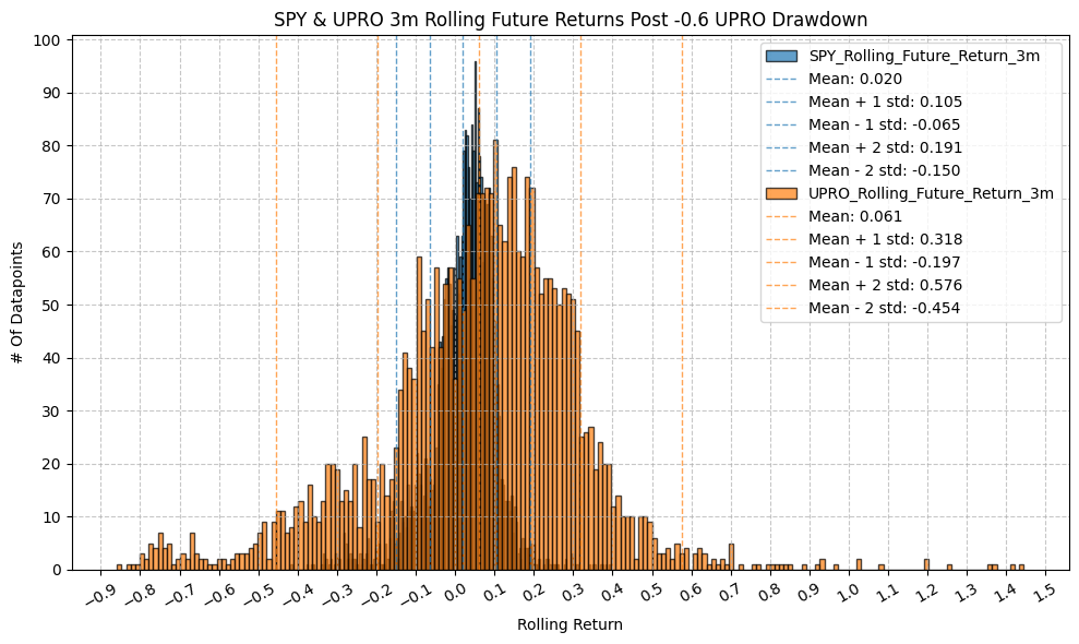

OLS Regression Results
=========================================================================================
Dep. Variable: UPRO_Rolling_Future_Return_3m R-squared: 0.977
Model: OLS Adj. R-squared: 0.977
Method: Least Squares F-statistic: 1.313e+05
Date: Mon, 23 Mar 2026 Prob (F-statistic): 0.00
Time: 22:04:09 Log-Likelihood: 5610.7
No. Observations: 3070 AIC: -1.122e+04
Df Residuals: 3068 BIC: -1.121e+04
Df Model: 1
Covariance Type: nonrobust
================================================================================================
coef std err t P>|t| [0.025 0.975]
------------------------------------------------------------------------------------------------
const 0.0004 0.001 0.593 0.553 -0.001 0.002
SPY_Rolling_Future_Return_3m 2.9877 0.008 362.353 0.000 2.972 3.004
==============================================================================
Omnibus: 1129.279 Durbin-Watson: 0.193
Prob(Omnibus): 0.000 Jarque-Bera (JB): 29406.672
Skew: 1.166 Prob(JB): 0.00
Kurtosis: 17.982 Cond. No. 11.7
==============================================================================
Notes:
[1] Standard Errors assume that the covariance matrix of the errors is correctly specified.
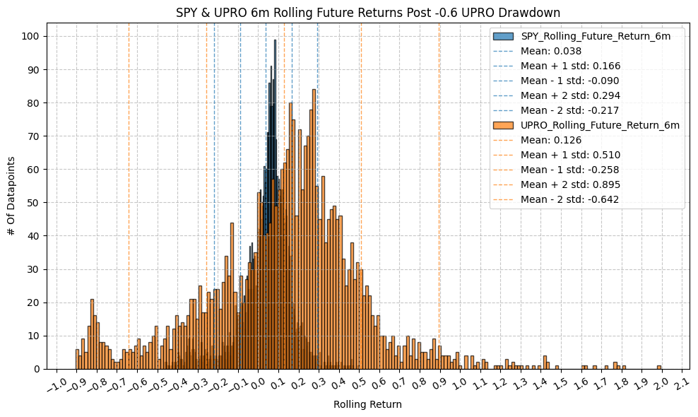
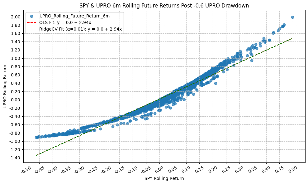
OLS Regression Results
=========================================================================================
Dep. Variable: UPRO_Rolling_Future_Return_6m R-squared: 0.956
Model: OLS Adj. R-squared: 0.956
Method: Least Squares F-statistic: 6.658e+04
Date: Mon, 23 Mar 2026 Prob (F-statistic): 0.00
Time: 22:04:11 Log-Likelihood: 3373.7
No. Observations: 3070 AIC: -6743.
Df Residuals: 3068 BIC: -6731.
Df Model: 1
Covariance Type: nonrobust
================================================================================================
coef std err t P>|t| [0.025 0.975]
------------------------------------------------------------------------------------------------
const 0.0138 0.002 9.065 0.000 0.011 0.017
SPY_Rolling_Future_Return_6m 2.9411 0.011 258.025 0.000 2.919 2.963
==============================================================================
Omnibus: 862.190 Durbin-Watson: 0.075
Prob(Omnibus): 0.000 Jarque-Bera (JB): 5062.816
Skew: 1.201 Prob(JB): 0.00
Kurtosis: 8.815 Cond. No. 7.84
==============================================================================
Notes:
[1] Standard Errors assume that the covariance matrix of the errors is correctly specified.
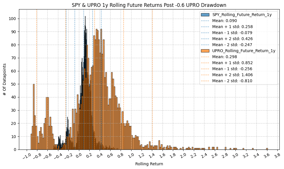
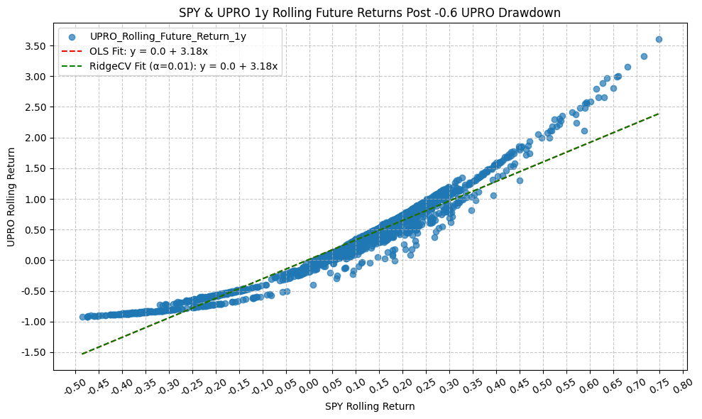
OLS Regression Results
=========================================================================================
Dep. Variable: UPRO_Rolling_Future_Return_1y R-squared: 0.932
Model: OLS Adj. R-squared: 0.932
Method: Least Squares F-statistic: 4.197e+04
Date: Mon, 23 Mar 2026 Prob (F-statistic): 0.00
Time: 22:04:12 Log-Likelihood: 1581.3
No. Observations: 3070 AIC: -3159.
Df Residuals: 3068 BIC: -3147.
Df Model: 1
Covariance Type: nonrobust
================================================================================================
coef std err t P>|t| [0.025 0.975]
------------------------------------------------------------------------------------------------
const 0.0132 0.003 4.455 0.000 0.007 0.019
SPY_Rolling_Future_Return_1y 3.1761 0.016 204.863 0.000 3.146 3.206
==============================================================================
Omnibus: 1211.105 Durbin-Watson: 0.065
Prob(Omnibus): 0.000 Jarque-Bera (JB): 10512.821
Skew: 1.634 Prob(JB): 0.00
Kurtosis: 11.456 Cond. No. 5.99
==============================================================================
Notes:
[1] Standard Errors assume that the covariance matrix of the errors is correctly specified.
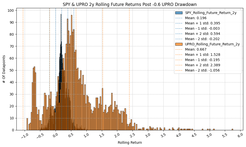
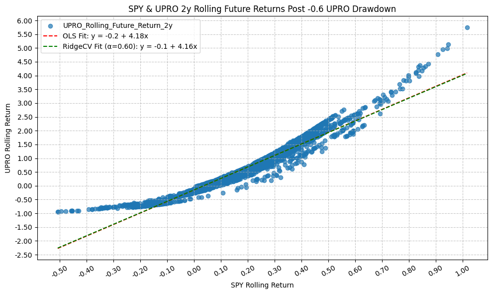
OLS Regression Results
=========================================================================================
Dep. Variable: UPRO_Rolling_Future_Return_2y R-squared: 0.932
Model: OLS Adj. R-squared: 0.932
Method: Least Squares F-statistic: 4.210e+04
Date: Mon, 23 Mar 2026 Prob (F-statistic): 0.00
Time: 22:04:14 Log-Likelihood: 230.84
No. Observations: 3070 AIC: -457.7
Df Residuals: 3068 BIC: -445.6
Df Model: 1
Covariance Type: nonrobust
================================================================================================
coef std err t P>|t| [0.025 0.975]
------------------------------------------------------------------------------------------------
const -0.1524 0.006 -26.790 0.000 -0.164 -0.141
SPY_Rolling_Future_Return_2y 4.1801 0.020 205.184 0.000 4.140 4.220
==============================================================================
Omnibus: 971.659 Durbin-Watson: 0.048
Prob(Omnibus): 0.000 Jarque-Bera (JB): 5572.803
Skew: 1.382 Prob(JB): 0.00
Kurtosis: 8.994 Cond. No. 5.23
==============================================================================
Notes:
[1] Standard Errors assume that the covariance matrix of the errors is correctly specified.
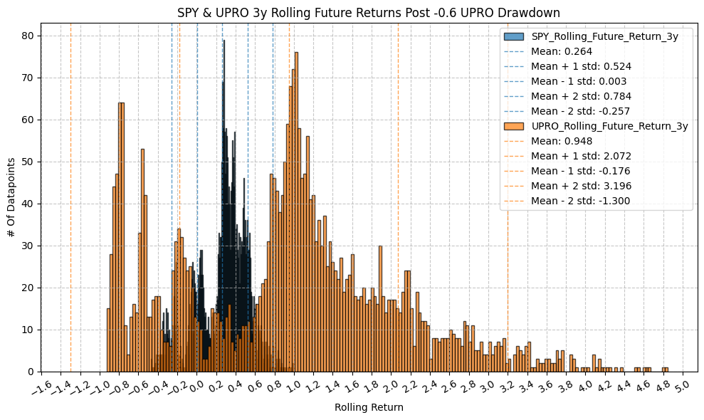
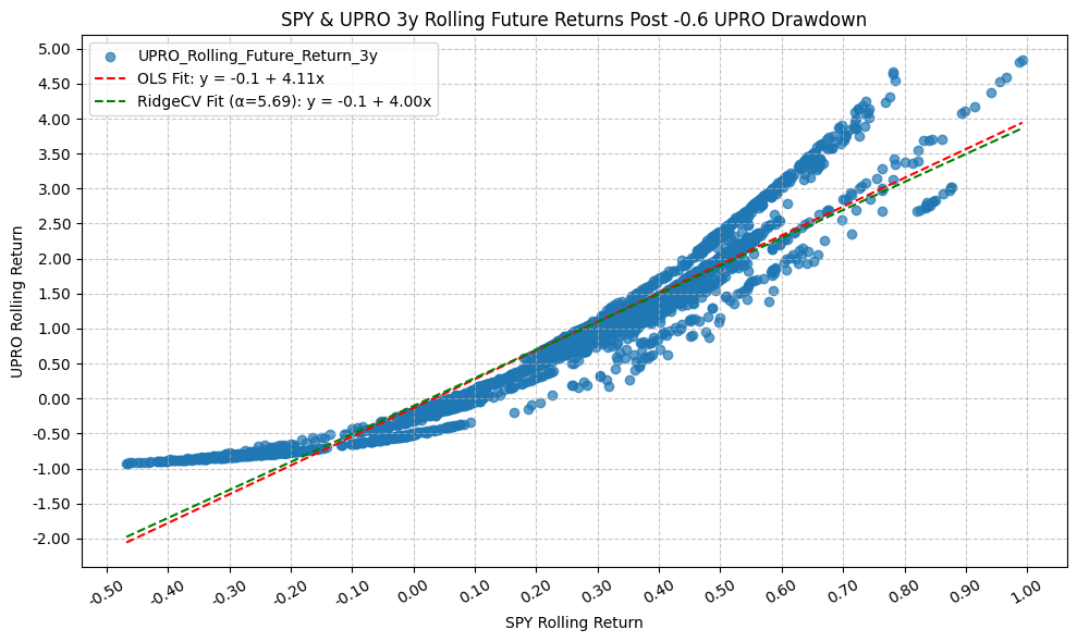
OLS Regression Results
=========================================================================================
Dep. Variable: UPRO_Rolling_Future_Return_3y R-squared: 0.906
Model: OLS Adj. R-squared: 0.906
Method: Least Squares F-statistic: 2.942e+04
Date: Mon, 23 Mar 2026 Prob (F-statistic): 0.00
Time: 22:04:16 Log-Likelihood: -1092.6
No. Observations: 3070 AIC: 2189.
Df Residuals: 3068 BIC: 2201.
Df Model: 1
Covariance Type: nonrobust
================================================================================================
coef std err t P>|t| [0.025 0.975]
------------------------------------------------------------------------------------------------
const -0.1351 0.009 -15.221 0.000 -0.152 -0.118
SPY_Rolling_Future_Return_3y 4.1098 0.024 171.516 0.000 4.063 4.157
==============================================================================
Omnibus: 523.502 Durbin-Watson: 0.022
Prob(Omnibus): 0.000 Jarque-Bera (JB): 948.375
Skew: 1.070 Prob(JB): 1.16e-206
Kurtosis: 4.683 Cond. No. 4.13
==============================================================================
Notes:
[1] Standard Errors assume that the covariance matrix of the errors is correctly specified.
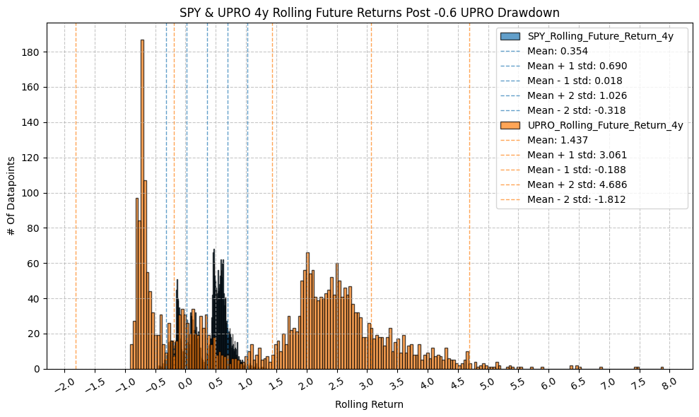
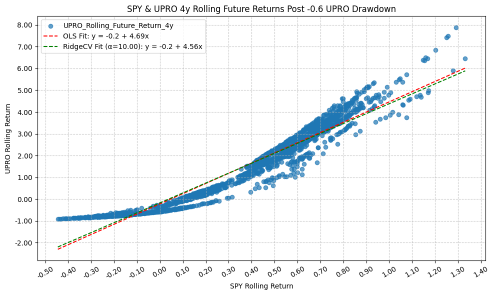
OLS Regression Results
=========================================================================================
Dep. Variable: UPRO_Rolling_Future_Return_4y R-squared: 0.942
Model: OLS Adj. R-squared: 0.942
Method: Least Squares F-statistic: 4.920e+04
Date: Mon, 23 Mar 2026 Prob (F-statistic): 0.00
Time: 22:04:18 Log-Likelihood: -1478.4
No. Observations: 3055 AIC: 2961.
Df Residuals: 3053 BIC: 2973.
Df Model: 1
Covariance Type: nonrobust
================================================================================================
coef std err t P>|t| [0.025 0.975]
------------------------------------------------------------------------------------------------
const -0.2228 0.010 -21.591 0.000 -0.243 -0.203
SPY_Rolling_Future_Return_4y 4.6896 0.021 221.805 0.000 4.648 4.731
==============================================================================
Omnibus: 120.374 Durbin-Watson: 0.033
Prob(Omnibus): 0.000 Jarque-Bera (JB): 311.607
Skew: 0.172 Prob(JB): 2.16e-68
Kurtosis: 4.526 Cond. No. 3.39
==============================================================================
Notes:
[1] Standard Errors assume that the covariance matrix of the errors is correctly specified.
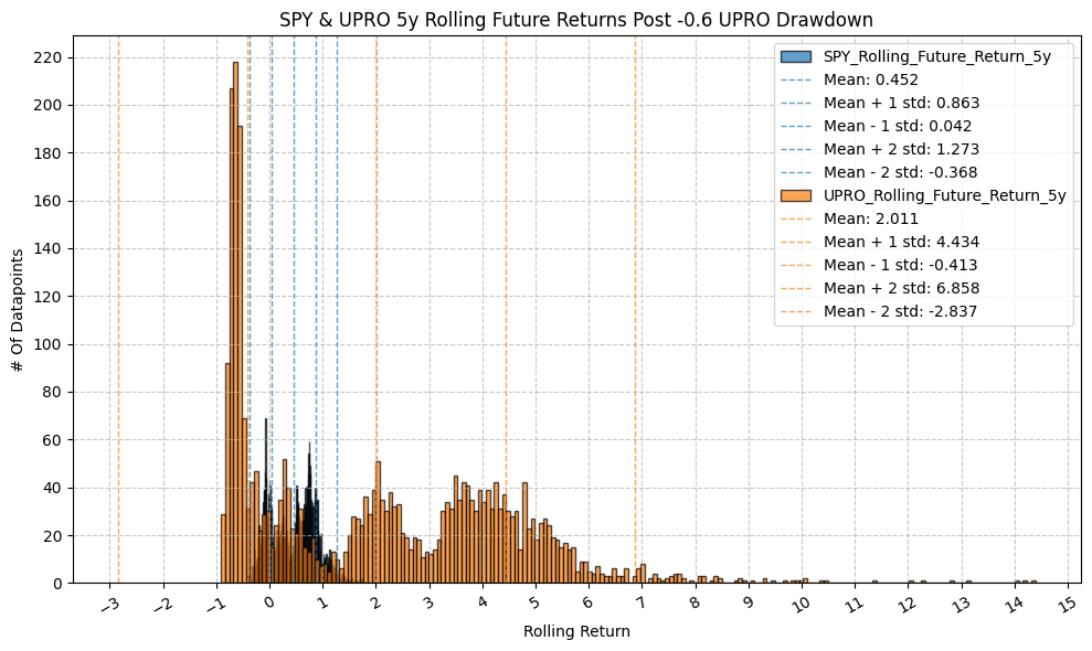
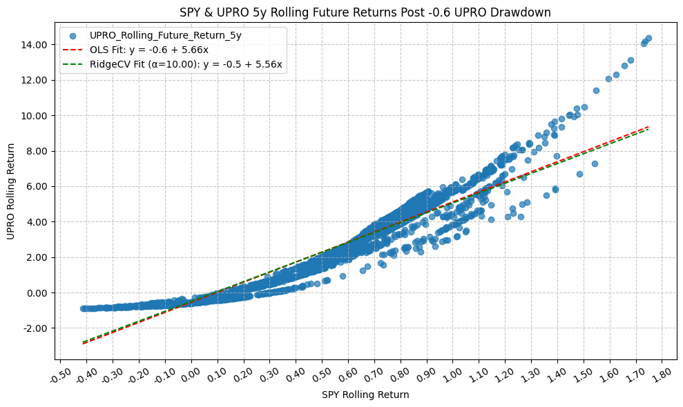
OLS Regression Results
=========================================================================================
Dep. Variable: UPRO_Rolling_Future_Return_5y R-squared: 0.919
Model: OLS Adj. R-squared: 0.919
Method: Least Squares F-statistic: 3.475e+04
Date: Mon, 23 Mar 2026 Prob (F-statistic): 0.00
Time: 22:04:20 Log-Likelihood: -3195.6
No. Observations: 3055 AIC: 6395.
Df Residuals: 3053 BIC: 6407.
Df Model: 1
Covariance Type: nonrobust
================================================================================================
coef std err t P>|t| [0.025 0.975]
------------------------------------------------------------------------------------------------
const -0.5516 0.019 -29.726 0.000 -0.588 -0.515
SPY_Rolling_Future_Return_5y 5.6648 0.030 186.402 0.000 5.605 5.724
==============================================================================
Omnibus: 454.815 Durbin-Watson: 0.025
Prob(Omnibus): 0.000 Jarque-Bera (JB): 2118.648
Skew: 0.640 Prob(JB): 0.00
Kurtosis: 6.874 Cond. No. 3.02
==============================================================================
Notes:
[1] Standard Errors assume that the covariance matrix of the errors is correctly specified.

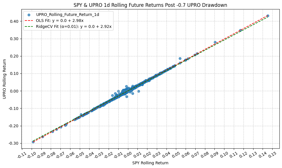
OLS Regression Results
=========================================================================================
Dep. Variable: UPRO_Rolling_Future_Return_1d R-squared: 0.997
Model: OLS Adj. R-squared: 0.997
Method: Least Squares F-statistic: 7.537e+05
Date: Mon, 23 Mar 2026 Prob (F-statistic): 0.00
Time: 22:04:21 Log-Likelihood: 10930.
No. Observations: 2365 AIC: -2.186e+04
Df Residuals: 2363 BIC: -2.184e+04
Df Model: 1
Covariance Type: nonrobust
================================================================================================
coef std err t P>|t| [0.025 0.975]
------------------------------------------------------------------------------------------------
const 8.912e-05 4.9e-05 1.819 0.069 -6.96e-06 0.000
SPY_Rolling_Future_Return_1d 2.9778 0.003 868.186 0.000 2.971 2.984
==============================================================================
Omnibus: 1557.950 Durbin-Watson: 2.718
Prob(Omnibus): 0.000 Jarque-Bera (JB): 638144.795
Skew: 1.869 Prob(JB): 0.00
Kurtosis: 83.386 Cond. No. 70.0
==============================================================================
Notes:
[1] Standard Errors assume that the covariance matrix of the errors is correctly specified.


OLS Regression Results
=========================================================================================
Dep. Variable: UPRO_Rolling_Future_Return_1w R-squared: 0.991
Model: OLS Adj. R-squared: 0.991
Method: Least Squares F-statistic: 2.714e+05
Date: Mon, 23 Mar 2026 Prob (F-statistic): 0.00
Time: 22:04:23 Log-Likelihood: 8089.4
No. Observations: 2365 AIC: -1.617e+04
Df Residuals: 2363 BIC: -1.616e+04
Df Model: 1
Covariance Type: nonrobust
================================================================================================
coef std err t P>|t| [0.025 0.975]
------------------------------------------------------------------------------------------------
const -7.259e-05 0.000 -0.445 0.656 -0.000 0.000
SPY_Rolling_Future_Return_1w 2.9630 0.006 520.956 0.000 2.952 2.974
==============================================================================
Omnibus: 893.071 Durbin-Watson: 1.046
Prob(Omnibus): 0.000 Jarque-Bera (JB): 167497.054
Skew: -0.620 Prob(JB): 0.00
Kurtosis: 44.209 Cond. No. 34.9
==============================================================================
Notes:
[1] Standard Errors assume that the covariance matrix of the errors is correctly specified.
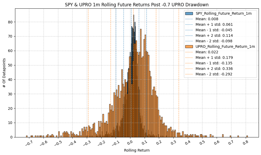

OLS Regression Results
=========================================================================================
Dep. Variable: UPRO_Rolling_Future_Return_1m R-squared: 0.984
Model: OLS Adj. R-squared: 0.984
Method: Least Squares F-statistic: 1.475e+05
Date: Mon, 23 Mar 2026 Prob (F-statistic): 0.00
Time: 22:04:25 Log-Likelihood: 5932.3
No. Observations: 2365 AIC: -1.186e+04
Df Residuals: 2363 BIC: -1.185e+04
Df Model: 1
Covariance Type: nonrobust
================================================================================================
coef std err t P>|t| [0.025 0.975]
------------------------------------------------------------------------------------------------
const -0.0007 0.000 -1.730 0.084 -0.002 9.44e-05
SPY_Rolling_Future_Return_1m 2.9413 0.008 384.062 0.000 2.926 2.956
==============================================================================
Omnibus: 954.674 Durbin-Watson: 0.364
Prob(Omnibus): 0.000 Jarque-Bera (JB): 63607.103
Skew: -1.055 Prob(JB): 0.00
Kurtosis: 28.319 Cond. No. 18.9
==============================================================================
Notes:
[1] Standard Errors assume that the covariance matrix of the errors is correctly specified.
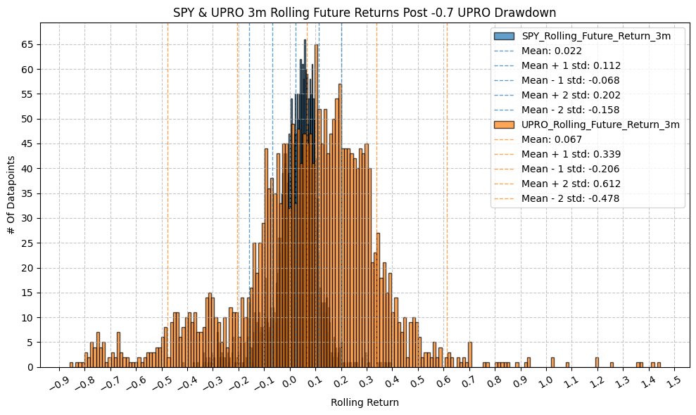
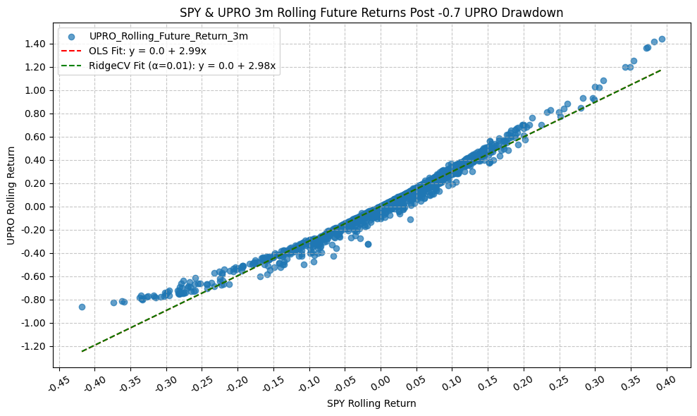
OLS Regression Results
=========================================================================================
Dep. Variable: UPRO_Rolling_Future_Return_3m R-squared: 0.976
Model: OLS Adj. R-squared: 0.976
Method: Least Squares F-statistic: 9.454e+04
Date: Mon, 23 Mar 2026 Prob (F-statistic): 0.00
Time: 22:04:26 Log-Likelihood: 4110.9
No. Observations: 2365 AIC: -8218.
Df Residuals: 2363 BIC: -8206.
Df Model: 1
Covariance Type: nonrobust
================================================================================================
coef std err t P>|t| [0.025 0.975]
------------------------------------------------------------------------------------------------
const 0.0012 0.001 1.377 0.169 -0.001 0.003
SPY_Rolling_Future_Return_3m 2.9865 0.010 307.478 0.000 2.967 3.006
==============================================================================
Omnibus: 813.501 Durbin-Watson: 0.169
Prob(Omnibus): 0.000 Jarque-Bera (JB): 16774.687
Skew: 1.111 Prob(JB): 0.00
Kurtosis: 15.856 Cond. No. 11.1
==============================================================================
Notes:
[1] Standard Errors assume that the covariance matrix of the errors is correctly specified.
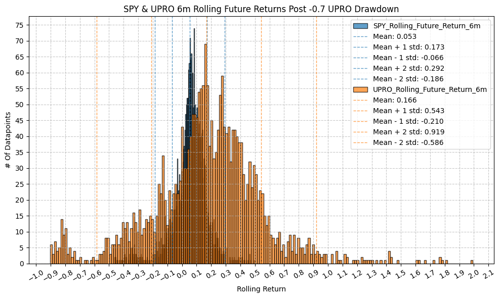
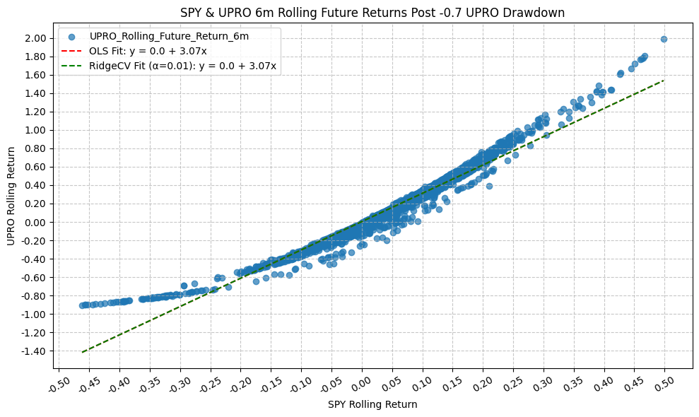
OLS Regression Results
=========================================================================================
Dep. Variable: UPRO_Rolling_Future_Return_6m R-squared: 0.954
Model: OLS Adj. R-squared: 0.954
Method: Least Squares F-statistic: 4.945e+04
Date: Mon, 23 Mar 2026 Prob (F-statistic): 0.00
Time: 22:04:28 Log-Likelihood: 2608.9
No. Observations: 2365 AIC: -5214.
Df Residuals: 2363 BIC: -5202.
Df Model: 1
Covariance Type: nonrobust
================================================================================================
coef std err t P>|t| [0.025 0.975]
------------------------------------------------------------------------------------------------
const 0.0035 0.002 1.919 0.055 -7.62e-05 0.007
SPY_Rolling_Future_Return_6m 3.0746 0.014 222.383 0.000 3.048 3.102
==============================================================================
Omnibus: 829.904 Durbin-Watson: 0.069
Prob(Omnibus): 0.000 Jarque-Bera (JB): 7402.181
Skew: 1.399 Prob(JB): 0.00
Kurtosis: 11.203 Cond. No. 8.39
==============================================================================
Notes:
[1] Standard Errors assume that the covariance matrix of the errors is correctly specified.

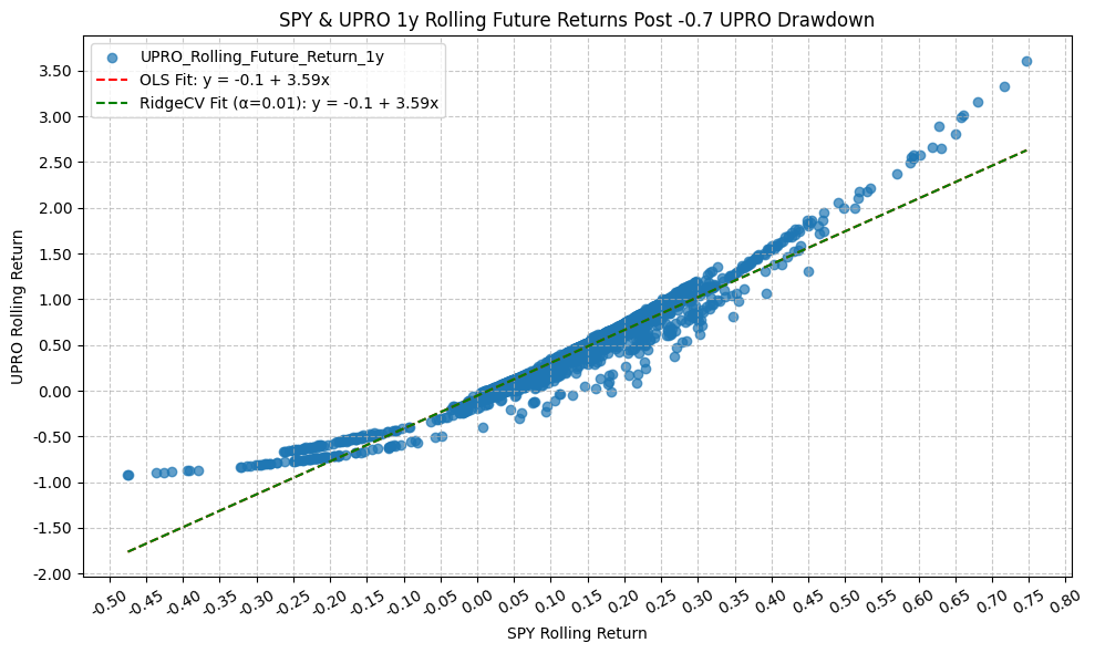
OLS Regression Results
=========================================================================================
Dep. Variable: UPRO_Rolling_Future_Return_1y R-squared: 0.941
Model: OLS Adj. R-squared: 0.941
Method: Least Squares F-statistic: 3.754e+04
Date: Mon, 23 Mar 2026 Prob (F-statistic): 0.00
Time: 22:04:30 Log-Likelihood: 1607.5
No. Observations: 2365 AIC: -3211.
Df Residuals: 2363 BIC: -3200.
Df Model: 1
Covariance Type: nonrobust
================================================================================================
coef std err t P>|t| [0.025 0.975]
------------------------------------------------------------------------------------------------
const -0.0550 0.003 -16.380 0.000 -0.062 -0.048
SPY_Rolling_Future_Return_1y 3.5927 0.019 193.753 0.000 3.556 3.629
==============================================================================
Omnibus: 724.967 Durbin-Watson: 0.076
Prob(Omnibus): 0.000 Jarque-Bera (JB): 11317.696
Skew: 1.018 Prob(JB): 0.00
Kurtosis: 13.522 Cond. No. 7.46
==============================================================================
Notes:
[1] Standard Errors assume that the covariance matrix of the errors is correctly specified.
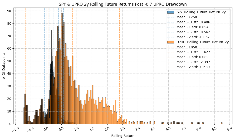
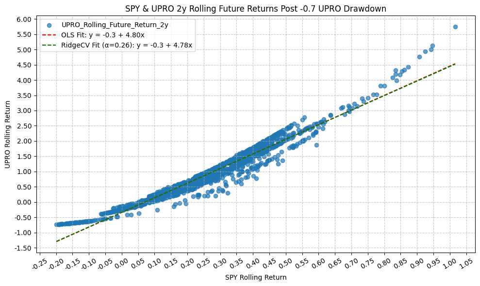
OLS Regression Results
=========================================================================================
Dep. Variable: UPRO_Rolling_Future_Return_2y R-squared: 0.947
Model: OLS Adj. R-squared: 0.947
Method: Least Squares F-statistic: 4.183e+04
Date: Mon, 23 Mar 2026 Prob (F-statistic): 0.00
Time: 22:04:31 Log-Likelihood: 728.42
No. Observations: 2365 AIC: -1453.
Df Residuals: 2363 BIC: -1441.
Df Model: 1
Covariance Type: nonrobust
================================================================================================
coef std err t P>|t| [0.025 0.975]
------------------------------------------------------------------------------------------------
const -0.3422 0.007 -49.480 0.000 -0.356 -0.329
SPY_Rolling_Future_Return_2y 4.7991 0.023 204.534 0.000 4.753 4.845
==============================================================================
Omnibus: 261.079 Durbin-Watson: 0.050
Prob(Omnibus): 0.000 Jarque-Bera (JB): 1786.755
Skew: -0.270 Prob(JB): 0.00
Kurtosis: 7.224 Cond. No. 6.82
==============================================================================
Notes:
[1] Standard Errors assume that the covariance matrix of the errors is correctly specified.
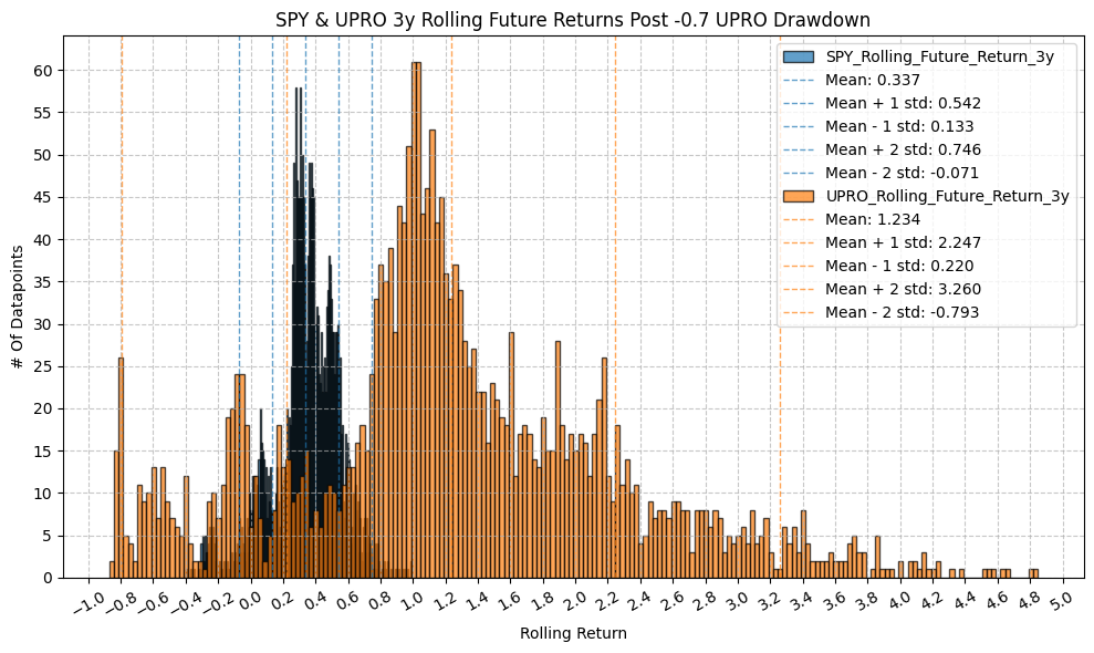
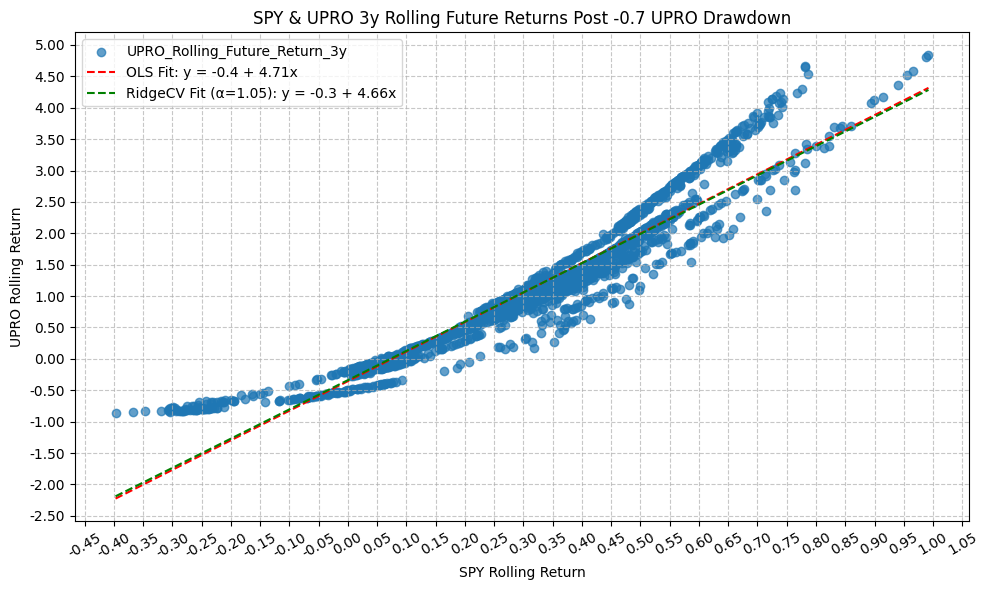
OLS Regression Results
=========================================================================================
Dep. Variable: UPRO_Rolling_Future_Return_3y R-squared: 0.901
Model: OLS Adj. R-squared: 0.901
Method: Least Squares F-statistic: 2.157e+04
Date: Mon, 23 Mar 2026 Prob (F-statistic): 0.00
Time: 22:04:33 Log-Likelihood: -648.61
No. Observations: 2365 AIC: 1301.
Df Residuals: 2363 BIC: 1313.
Df Model: 1
Covariance Type: nonrobust
================================================================================================
coef std err t P>|t| [0.025 0.975]
------------------------------------------------------------------------------------------------
const -0.3554 0.013 -28.106 0.000 -0.380 -0.331
SPY_Rolling_Future_Return_3y 4.7080 0.032 146.881 0.000 4.645 4.771
==============================================================================
Omnibus: 350.131 Durbin-Watson: 0.028
Prob(Omnibus): 0.000 Jarque-Bera (JB): 725.354
Skew: 0.885 Prob(JB): 3.10e-158
Kurtosis: 5.056 Cond. No. 5.47
==============================================================================
Notes:
[1] Standard Errors assume that the covariance matrix of the errors is correctly specified.
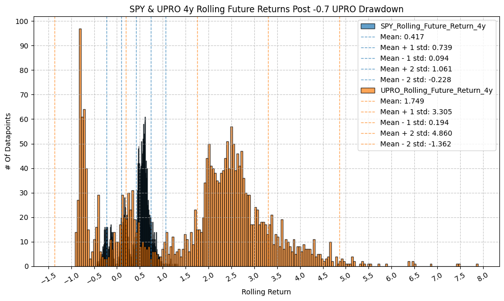
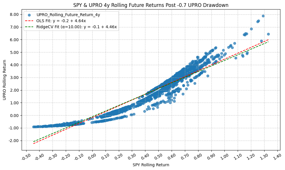
OLS Regression Results
=========================================================================================
Dep. Variable: UPRO_Rolling_Future_Return_4y R-squared: 0.925
Model: OLS Adj. R-squared: 0.925
Method: Least Squares F-statistic: 2.909e+04
Date: Mon, 23 Mar 2026 Prob (F-statistic): 0.00
Time: 22:04:35 Log-Likelihood: -1339.1
No. Observations: 2365 AIC: 2682.
Df Residuals: 2363 BIC: 2694.
Df Model: 1
Covariance Type: nonrobust
================================================================================================
coef std err t P>|t| [0.025 0.975]
------------------------------------------------------------------------------------------------
const -0.1851 0.014 -12.911 0.000 -0.213 -0.157
SPY_Rolling_Future_Return_4y 4.6424 0.027 170.562 0.000 4.589 4.696
==============================================================================
Omnibus: 55.440 Durbin-Watson: 0.030
Prob(Omnibus): 0.000 Jarque-Bera (JB): 118.149
Skew: 0.081 Prob(JB): 2.21e-26
Kurtosis: 4.083 Cond. No. 3.69
==============================================================================
Notes:
[1] Standard Errors assume that the covariance matrix of the errors is correctly specified.
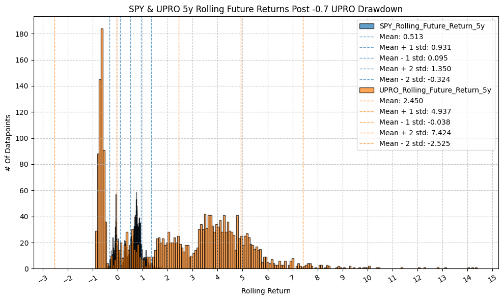
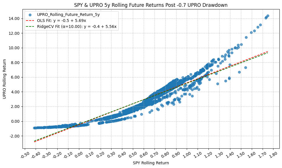
OLS Regression Results
=========================================================================================
Dep. Variable: UPRO_Rolling_Future_Return_5y R-squared: 0.917
Model: OLS Adj. R-squared: 0.917
Method: Least Squares F-statistic: 2.615e+04
Date: Mon, 23 Mar 2026 Prob (F-statistic): 0.00
Time: 22:04:37 Log-Likelihood: -2565.1
No. Observations: 2365 AIC: 5134.
Df Residuals: 2363 BIC: 5146.
Df Model: 1
Covariance Type: nonrobust
================================================================================================
coef std err t P>|t| [0.025 0.975]
------------------------------------------------------------------------------------------------
const -0.4704 0.023 -20.189 0.000 -0.516 -0.425
SPY_Rolling_Future_Return_5y 5.6929 0.035 161.724 0.000 5.624 5.762
==============================================================================
Omnibus: 310.928 Durbin-Watson: 0.028
Prob(Omnibus): 0.000 Jarque-Bera (JB): 1361.563
Skew: 0.566 Prob(JB): 2.19e-296
Kurtosis: 6.541 Cond. No. 3.12
==============================================================================
Notes:
[1] Standard Errors assume that the covariance matrix of the errors is correctly specified.
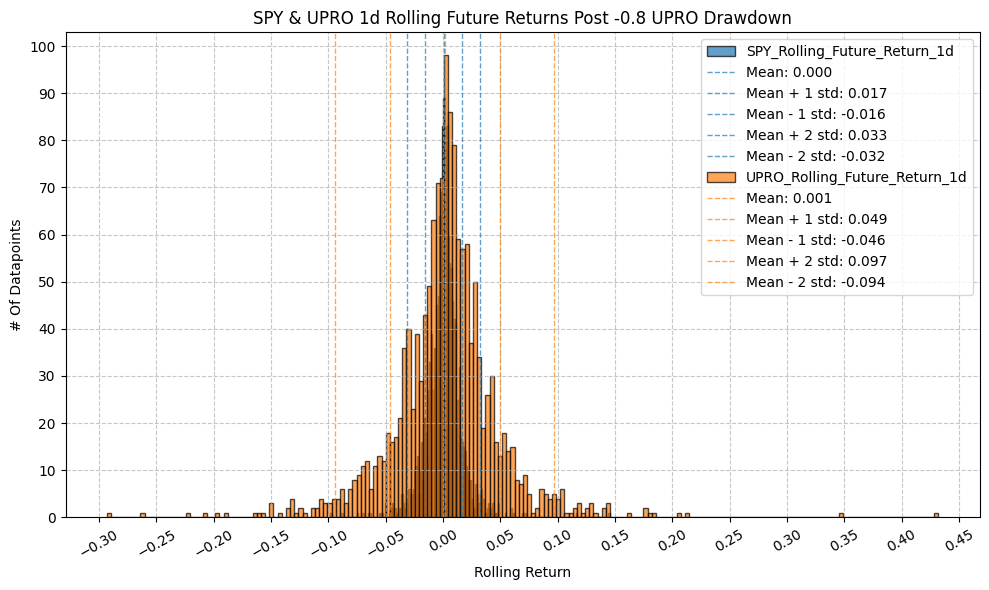
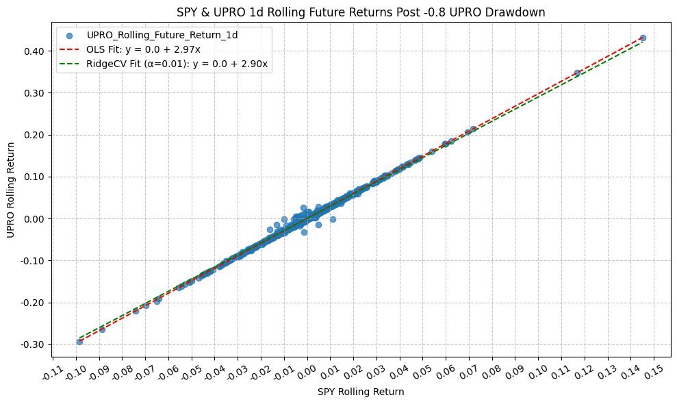
OLS Regression Results
=========================================================================================
Dep. Variable: UPRO_Rolling_Future_Return_1d R-squared: 0.997
Model: OLS Adj. R-squared: 0.997
Method: Least Squares F-statistic: 4.359e+05
Date: Mon, 23 Mar 2026 Prob (F-statistic): 0.00
Time: 22:04:39 Log-Likelihood: 6602.3
No. Observations: 1478 AIC: -1.320e+04
Df Residuals: 1476 BIC: -1.319e+04
Df Model: 1
Covariance Type: nonrobust
================================================================================================
coef std err t P>|t| [0.025 0.975]
------------------------------------------------------------------------------------------------
const 0.0001 7.23e-05 1.542 0.123 -3.04e-05 0.000
SPY_Rolling_Future_Return_1d 2.9735 0.005 660.239 0.000 2.965 2.982
==============================================================================
Omnibus: 758.954 Durbin-Watson: 2.689
Prob(Omnibus): 0.000 Jarque-Bera (JB): 237432.928
Skew: 1.143 Prob(JB): 0.00
Kurtosis: 65.050 Cond. No. 62.3
==============================================================================
Notes:
[1] Standard Errors assume that the covariance matrix of the errors is correctly specified.
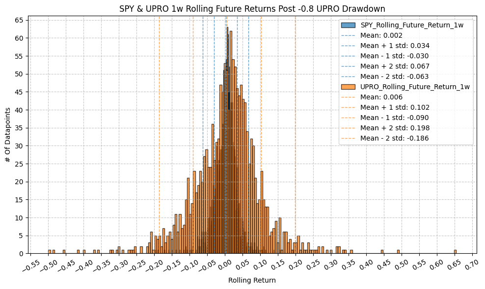
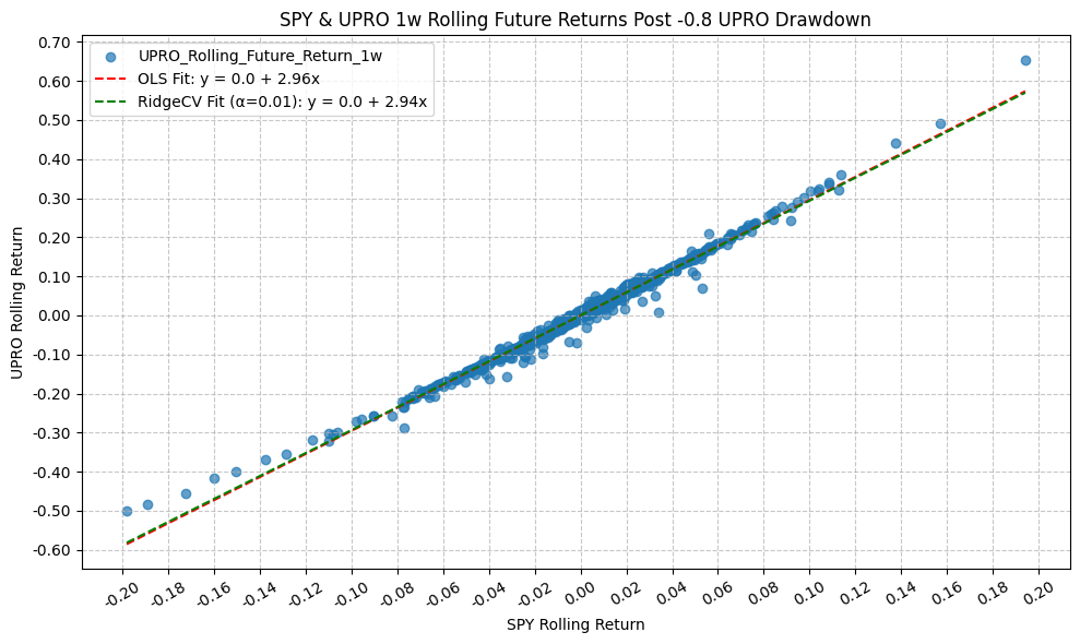
OLS Regression Results
=========================================================================================
Dep. Variable: UPRO_Rolling_Future_Return_1w R-squared: 0.990
Model: OLS Adj. R-squared: 0.990
Method: Least Squares F-statistic: 1.474e+05
Date: Mon, 23 Mar 2026 Prob (F-statistic): 0.00
Time: 22:04:40 Log-Likelihood: 4775.7
No. Observations: 1478 AIC: -9547.
Df Residuals: 1476 BIC: -9537.
Df Model: 1
Covariance Type: nonrobust
================================================================================================
coef std err t P>|t| [0.025 0.975]
------------------------------------------------------------------------------------------------
const 4.459e-06 0.000 0.018 0.986 -0.000 0.000
SPY_Rolling_Future_Return_1w 2.9571 0.008 383.898 0.000 2.942 2.972
==============================================================================
Omnibus: 517.395 Durbin-Watson: 1.023
Prob(Omnibus): 0.000 Jarque-Bera (JB): 52529.136
Skew: -0.625 Prob(JB): 0.00
Kurtosis: 32.179 Cond. No. 31.0
==============================================================================
Notes:
[1] Standard Errors assume that the covariance matrix of the errors is correctly specified.
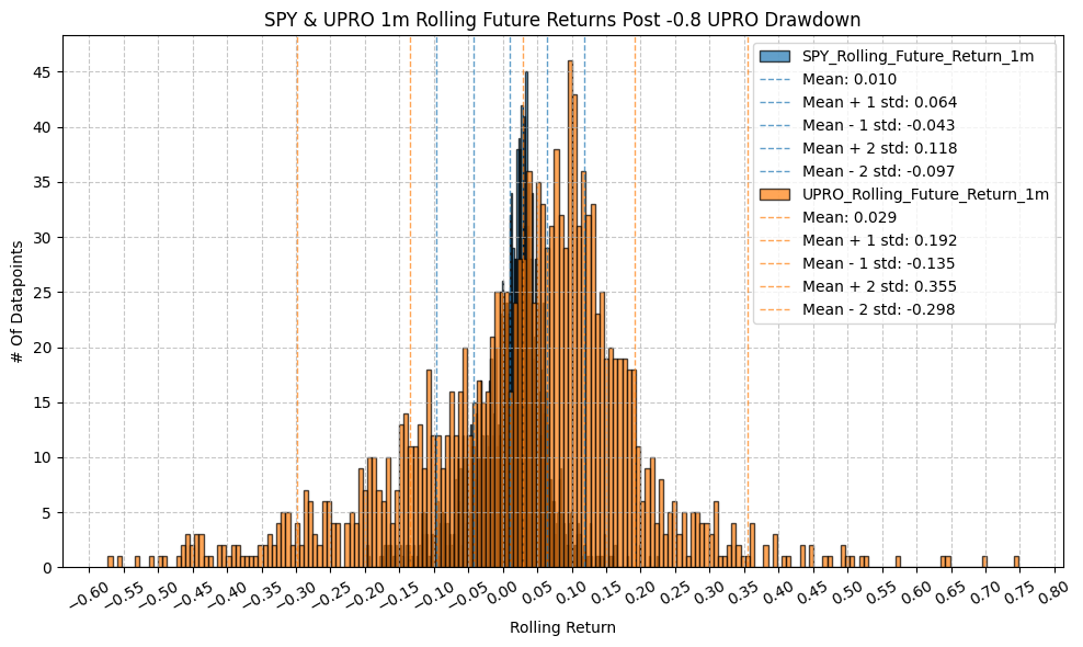
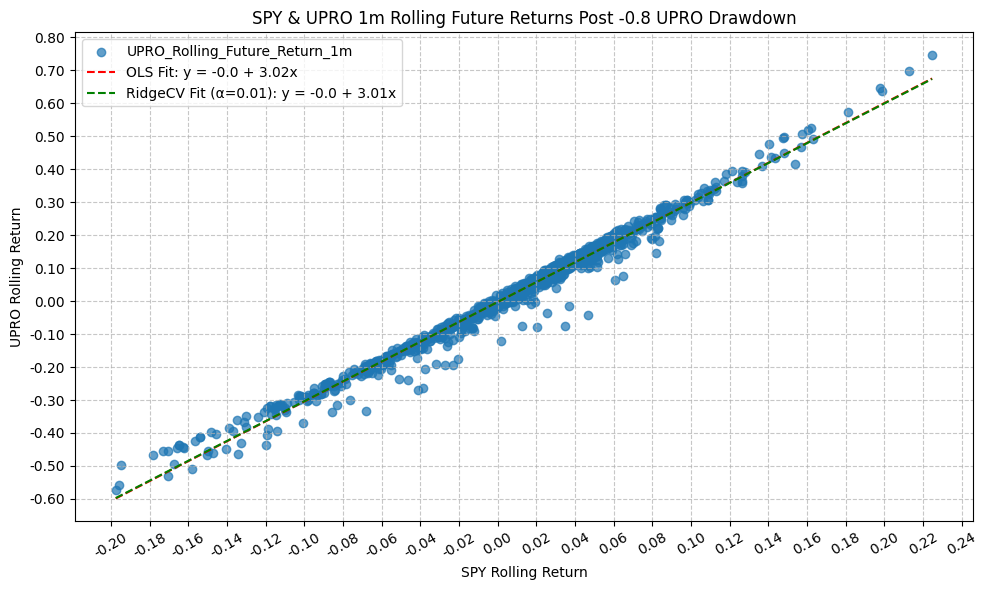
OLS Regression Results
=========================================================================================
Dep. Variable: UPRO_Rolling_Future_Return_1m R-squared: 0.983
Model: OLS Adj. R-squared: 0.983
Method: Least Squares F-statistic: 8.446e+04
Date: Mon, 23 Mar 2026 Prob (F-statistic): 0.00
Time: 22:04:42 Log-Likelihood: 3586.0
No. Observations: 1478 AIC: -7168.
Df Residuals: 1476 BIC: -7157.
Df Model: 1
Covariance Type: nonrobust
================================================================================================
coef std err t P>|t| [0.025 0.975]
------------------------------------------------------------------------------------------------
const -0.0029 0.001 -5.070 0.000 -0.004 -0.002
SPY_Rolling_Future_Return_1m 3.0166 0.010 290.618 0.000 2.996 3.037
==============================================================================
Omnibus: 950.759 Durbin-Watson: 0.291
Prob(Omnibus): 0.000 Jarque-Bera (JB): 19698.886
Skew: -2.648 Prob(JB): 0.00
Kurtosis: 20.083 Cond. No. 18.7
==============================================================================
Notes:
[1] Standard Errors assume that the covariance matrix of the errors is correctly specified.
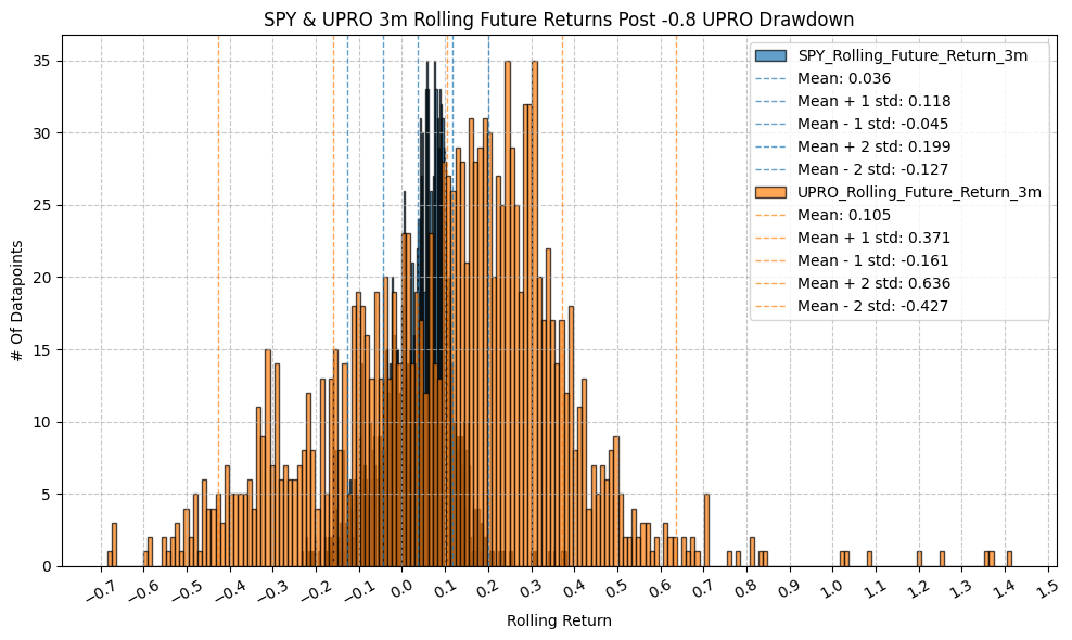
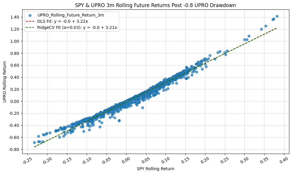
OLS Regression Results
=========================================================================================
Dep. Variable: UPRO_Rolling_Future_Return_3m R-squared: 0.980
Model: OLS Adj. R-squared: 0.980
Method: Least Squares F-statistic: 7.176e+04
Date: Mon, 23 Mar 2026 Prob (F-statistic): 0.00
Time: 22:04:43 Log-Likelihood: 2747.3
No. Observations: 1478 AIC: -5491.
Df Residuals: 1476 BIC: -5480.
Df Model: 1
Covariance Type: nonrobust
================================================================================================
coef std err t P>|t| [0.025 0.975]
------------------------------------------------------------------------------------------------
const -0.0120 0.001 -11.211 0.000 -0.014 -0.010
SPY_Rolling_Future_Return_3m 3.2237 0.012 267.883 0.000 3.200 3.247
==============================================================================
Omnibus: 396.131 Durbin-Watson: 0.203
Prob(Omnibus): 0.000 Jarque-Bera (JB): 3161.615
Skew: -1.020 Prob(JB): 0.00
Kurtosis: 9.868 Cond. No. 12.3
==============================================================================
Notes:
[1] Standard Errors assume that the covariance matrix of the errors is correctly specified.
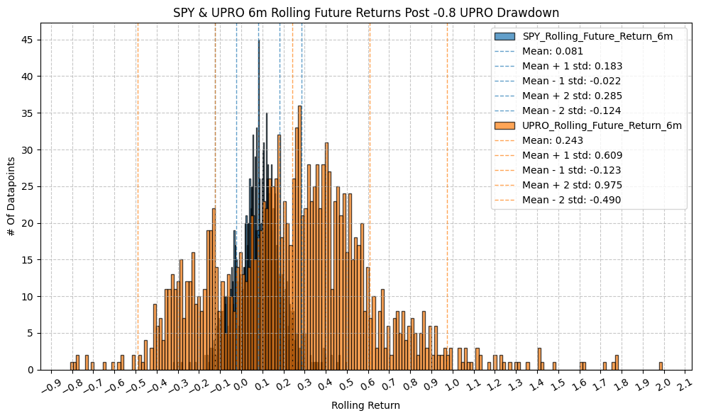
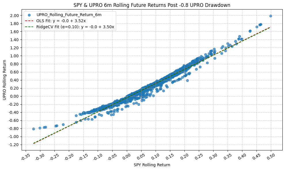
OLS Regression Results
=========================================================================================
Dep. Variable: UPRO_Rolling_Future_Return_6m R-squared: 0.971
Model: OLS Adj. R-squared: 0.971
Method: Least Squares F-statistic: 4.870e+04
Date: Mon, 23 Mar 2026 Prob (F-statistic): 0.00
Time: 22:04:45 Log-Likelihood: 1994.5
No. Observations: 1478 AIC: -3985.
Df Residuals: 1476 BIC: -3974.
Df Model: 1
Covariance Type: nonrobust
================================================================================================
coef std err t P>|t| [0.025 0.975]
------------------------------------------------------------------------------------------------
const -0.0410 0.002 -19.749 0.000 -0.045 -0.037
SPY_Rolling_Future_Return_6m 3.5209 0.016 220.689 0.000 3.490 3.552
==============================================================================
Omnibus: 302.897 Durbin-Watson: 0.139
Prob(Omnibus): 0.000 Jarque-Bera (JB): 1793.969
Skew: -0.817 Prob(JB): 0.00
Kurtosis: 8.144 Cond. No. 9.83
==============================================================================
Notes:
[1] Standard Errors assume that the covariance matrix of the errors is correctly specified.
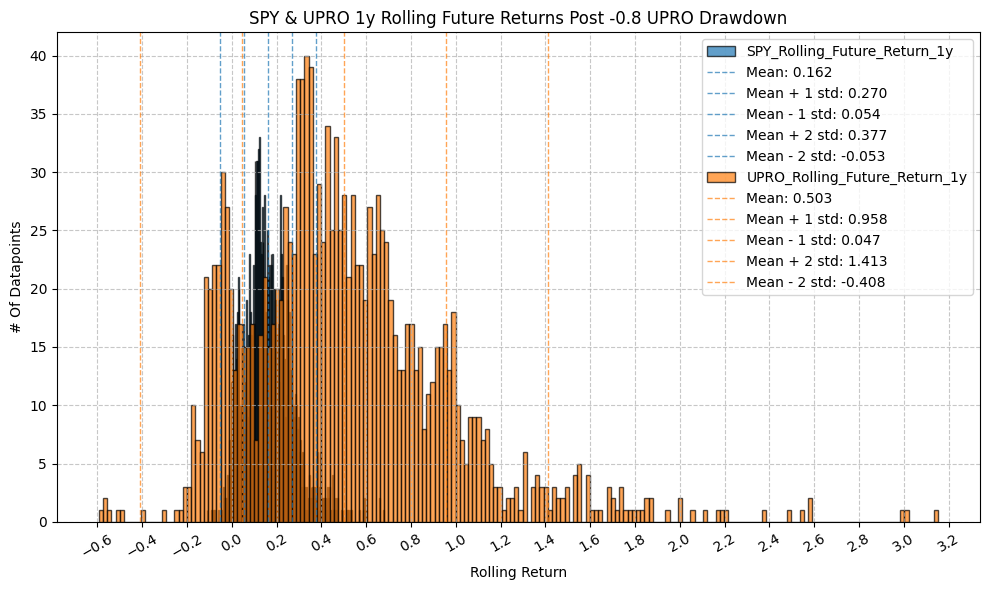
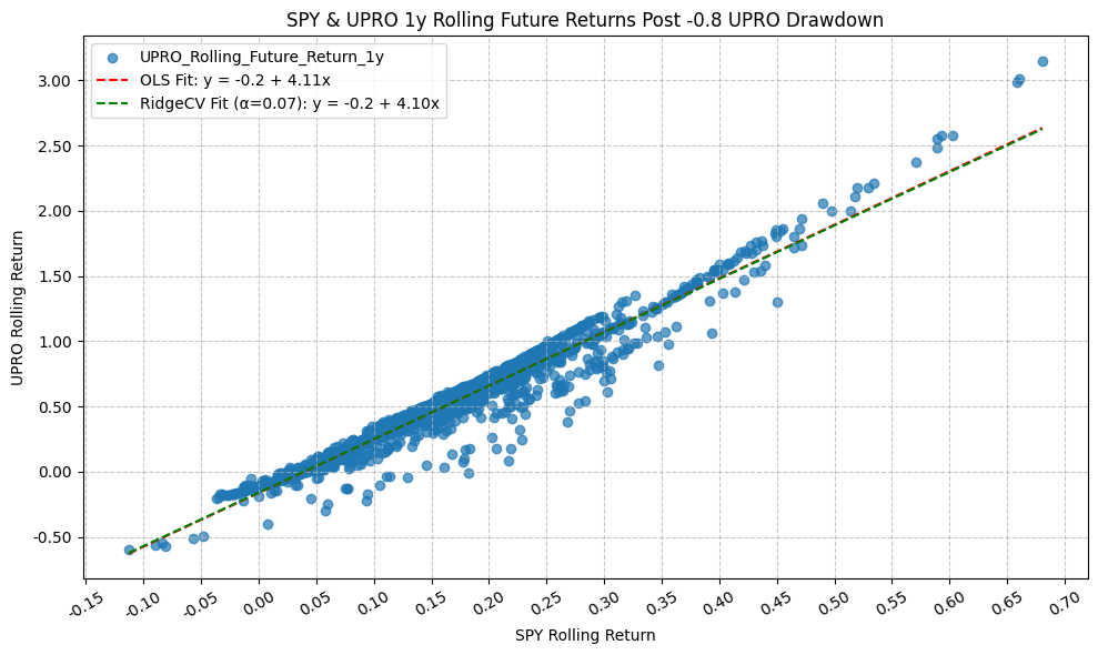
OLS Regression Results
=========================================================================================
Dep. Variable: UPRO_Rolling_Future_Return_1y R-squared: 0.945
Model: OLS Adj. R-squared: 0.945
Method: Least Squares F-statistic: 2.530e+04
Date: Mon, 23 Mar 2026 Prob (F-statistic): 0.00
Time: 22:04:47 Log-Likelihood: 1207.7
No. Observations: 1478 AIC: -2411.
Df Residuals: 1476 BIC: -2401.
Df Model: 1
Covariance Type: nonrobust
================================================================================================
coef std err t P>|t| [0.025 0.975]
------------------------------------------------------------------------------------------------
const -0.1638 0.005 -32.561 0.000 -0.174 -0.154
SPY_Rolling_Future_Return_1y 4.1147 0.026 159.048 0.000 4.064 4.165
==============================================================================
Omnibus: 635.689 Durbin-Watson: 0.055
Prob(Omnibus): 0.000 Jarque-Bera (JB): 4011.205
Skew: -1.899 Prob(JB): 0.00
Kurtosis: 10.121 Cond. No. 9.55
==============================================================================
Notes:
[1] Standard Errors assume that the covariance matrix of the errors is correctly specified.
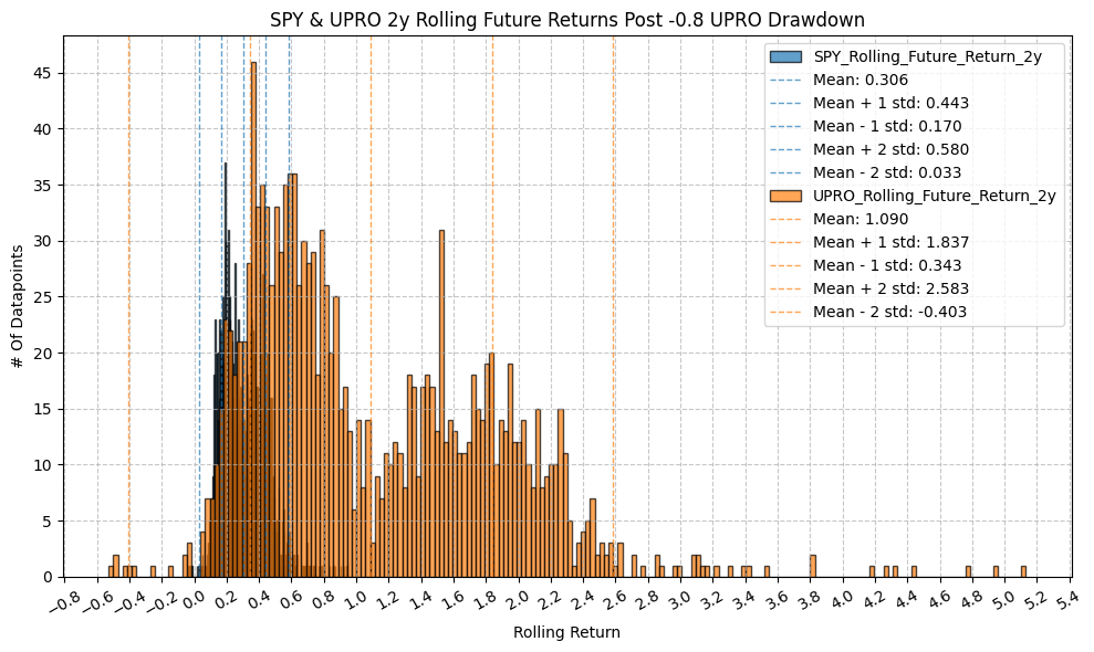
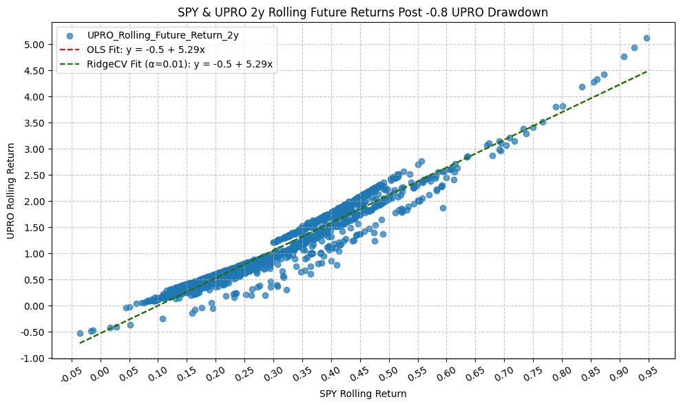
OLS Regression Results
=========================================================================================
Dep. Variable: UPRO_Rolling_Future_Return_2y R-squared: 0.940
Model: OLS Adj. R-squared: 0.940
Method: Least Squares F-statistic: 2.321e+04
Date: Mon, 23 Mar 2026 Prob (F-statistic): 0.00
Time: 22:04:48 Log-Likelihood: 416.77
No. Observations: 1478 AIC: -829.5
Df Residuals: 1476 BIC: -818.9
Df Model: 1
Covariance Type: nonrobust
================================================================================================
coef std err t P>|t| [0.025 0.975]
------------------------------------------------------------------------------------------------
const -0.5307 0.012 -45.547 0.000 -0.554 -0.508
SPY_Rolling_Future_Return_2y 5.2902 0.035 152.339 0.000 5.222 5.358
==============================================================================
Omnibus: 349.846 Durbin-Watson: 0.045
Prob(Omnibus): 0.000 Jarque-Bera (JB): 913.818
Skew: -1.242 Prob(JB): 3.69e-199
Kurtosis: 5.944 Cond. No. 8.01
==============================================================================
Notes:
[1] Standard Errors assume that the covariance matrix of the errors is correctly specified.
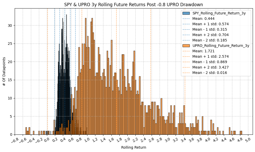
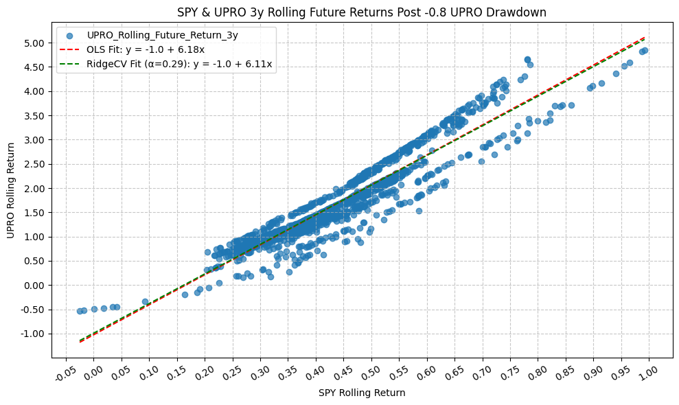
OLS Regression Results
=========================================================================================
Dep. Variable: UPRO_Rolling_Future_Return_3y R-squared: 0.884
Model: OLS Adj. R-squared: 0.884
Method: Least Squares F-statistic: 1.127e+04
Date: Mon, 23 Mar 2026 Prob (F-statistic): 0.00
Time: 22:04:50 Log-Likelihood: -267.99
No. Observations: 1478 AIC: 540.0
Df Residuals: 1476 BIC: 550.6
Df Model: 1
Covariance Type: nonrobust
================================================================================================
coef std err t P>|t| [0.025 0.975]
------------------------------------------------------------------------------------------------
const -1.0261 0.027 -38.067 0.000 -1.079 -0.973
SPY_Rolling_Future_Return_3y 6.1824 0.058 106.180 0.000 6.068 6.297
==============================================================================
Omnibus: 75.072 Durbin-Watson: 0.032
Prob(Omnibus): 0.000 Jarque-Bera (JB): 91.613
Skew: -0.514 Prob(JB): 1.28e-20
Kurtosis: 3.657 Cond. No. 9.26
==============================================================================
Notes:
[1] Standard Errors assume that the covariance matrix of the errors is correctly specified.
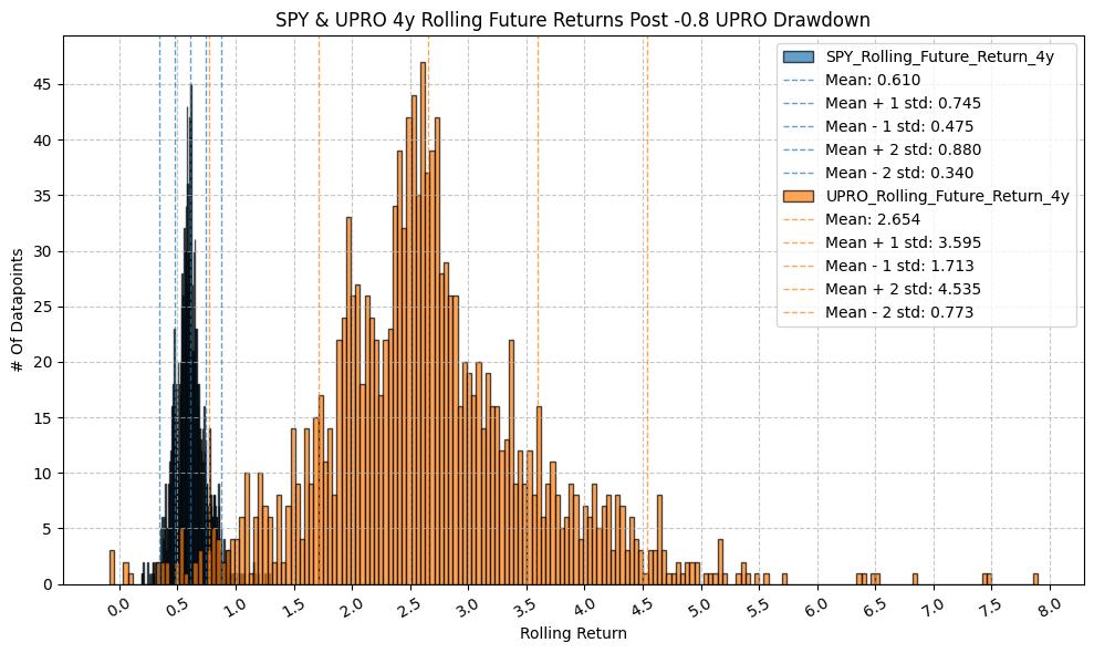
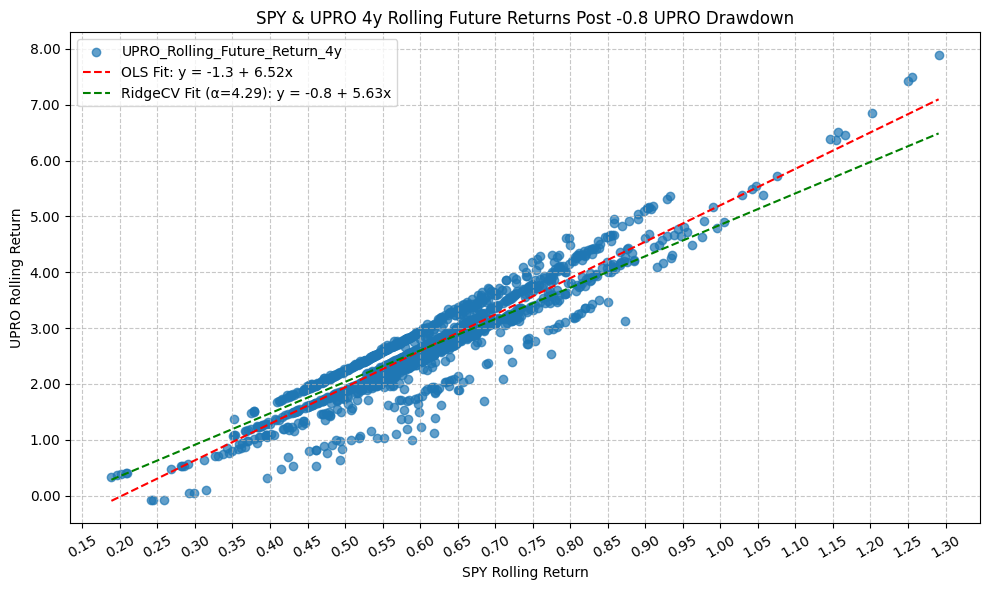
OLS Regression Results
=========================================================================================
Dep. Variable: UPRO_Rolling_Future_Return_4y R-squared: 0.877
Model: OLS Adj. R-squared: 0.877
Method: Least Squares F-statistic: 1.049e+04
Date: Mon, 23 Mar 2026 Prob (F-statistic): 0.00
Time: 22:04:52 Log-Likelihood: -459.80
No. Observations: 1478 AIC: 923.6
Df Residuals: 1476 BIC: 934.2
Df Model: 1
Covariance Type: nonrobust
================================================================================================
coef std err t P>|t| [0.025 0.975]
------------------------------------------------------------------------------------------------
const -1.3239 0.040 -33.279 0.000 -1.402 -1.246
SPY_Rolling_Future_Return_4y 6.5226 0.064 102.410 0.000 6.398 6.648
==============================================================================
Omnibus: 316.447 Durbin-Watson: 0.032
Prob(Omnibus): 0.000 Jarque-Bera (JB): 744.845
Skew: -1.168 Prob(JB): 1.82e-162
Kurtosis: 5.577 Cond. No. 10.2
==============================================================================
Notes:
[1] Standard Errors assume that the covariance matrix of the errors is correctly specified.
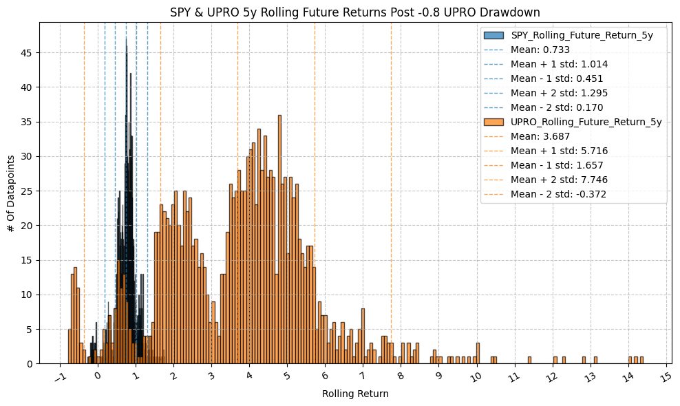
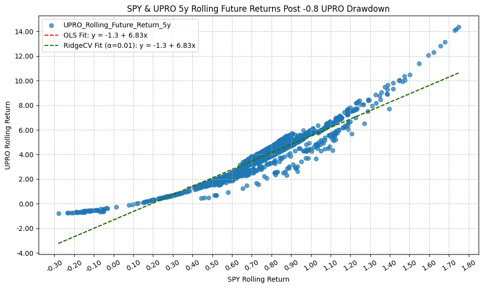
OLS Regression Results
=========================================================================================
Dep. Variable: UPRO_Rolling_Future_Return_5y R-squared: 0.895
Model: OLS Adj. R-squared: 0.895
Method: Least Squares F-statistic: 1.257e+04
Date: Mon, 23 Mar 2026 Prob (F-statistic): 0.00
Time: 22:04:53 Log-Likelihood: -1477.7
No. Observations: 1478 AIC: 2959.
Df Residuals: 1476 BIC: 2970.
Df Model: 1
Covariance Type: nonrobust
================================================================================================
coef std err t P>|t| [0.025 0.975]
------------------------------------------------------------------------------------------------
const -1.3148 0.048 -27.521 0.000 -1.409 -1.221
SPY_Rolling_Future_Return_5y 6.8269 0.061 112.133 0.000 6.707 6.946
==============================================================================
Omnibus: 180.837 Durbin-Watson: 0.042
Prob(Omnibus): 0.000 Jarque-Bera (JB): 811.822
Skew: 0.496 Prob(JB): 5.19e-177
Kurtosis: 6.492 Cond. No. 5.57
==============================================================================
Notes:
[1] Standard Errors assume that the covariance matrix of the errors is correctly specified.
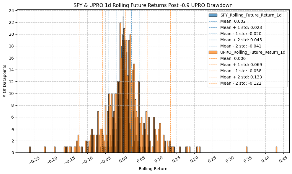
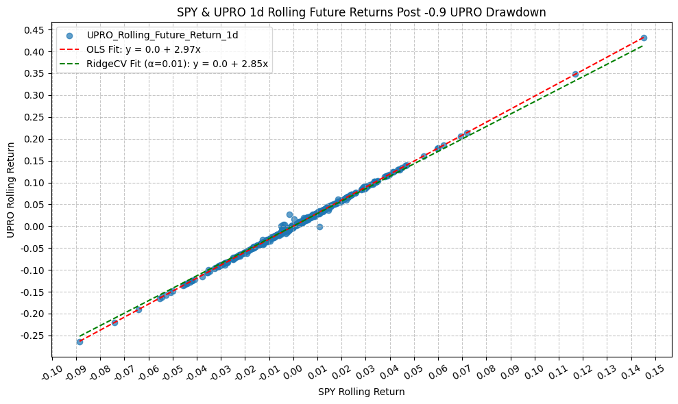
OLS Regression Results
=========================================================================================
Dep. Variable: UPRO_Rolling_Future_Return_1d R-squared: 0.998
Model: OLS Adj. R-squared: 0.998
Method: Least Squares F-statistic: 2.296e+05
Date: Mon, 23 Mar 2026 Prob (F-statistic): 0.00
Time: 22:04:55 Log-Likelihood: 2166.7
No. Observations: 491 AIC: -4329.
Df Residuals: 489 BIC: -4321.
Df Model: 1
Covariance Type: nonrobust
================================================================================================
coef std err t P>|t| [0.025 0.975]
------------------------------------------------------------------------------------------------
const 0.0001 0.000 0.842 0.400 -0.000 0.000
SPY_Rolling_Future_Return_1d 2.9736 0.006 479.155 0.000 2.961 2.986
==============================================================================
Omnibus: 206.818 Durbin-Watson: 2.771
Prob(Omnibus): 0.000 Jarque-Bera (JB): 96271.874
Skew: 0.202 Prob(JB): 0.00
Kurtosis: 71.597 Cond. No. 46.8
==============================================================================
Notes:
[1] Standard Errors assume that the covariance matrix of the errors is correctly specified.
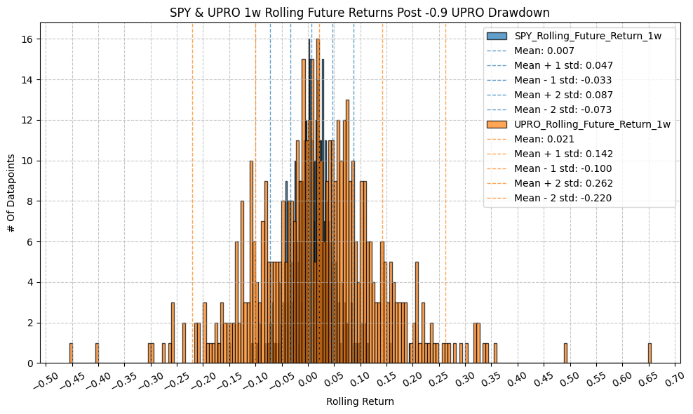
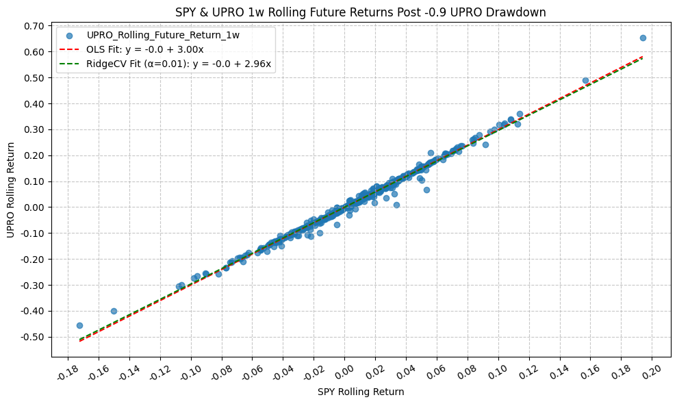
OLS Regression Results
=========================================================================================
Dep. Variable: UPRO_Rolling_Future_Return_1w R-squared: 0.990
Model: OLS Adj. R-squared: 0.990
Method: Least Squares F-statistic: 4.746e+04
Date: Mon, 23 Mar 2026 Prob (F-statistic): 0.00
Time: 22:04:57 Log-Likelihood: 1468.0
No. Observations: 491 AIC: -2932.
Df Residuals: 489 BIC: -2924.
Df Model: 1
Covariance Type: nonrobust
================================================================================================
coef std err t P>|t| [0.025 0.975]
------------------------------------------------------------------------------------------------
const -0.0009 0.001 -1.609 0.108 -0.002 0.000
SPY_Rolling_Future_Return_1w 2.9980 0.014 217.862 0.000 2.971 3.025
==============================================================================
Omnibus: 245.324 Durbin-Watson: 1.337
Prob(Omnibus): 0.000 Jarque-Bera (JB): 7331.985
Skew: -1.554 Prob(JB): 0.00
Kurtosis: 21.674 Cond. No. 25.0
==============================================================================
Notes:
[1] Standard Errors assume that the covariance matrix of the errors is correctly specified.
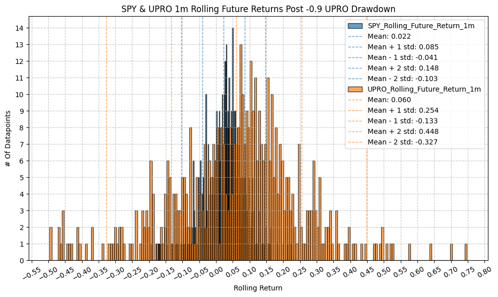
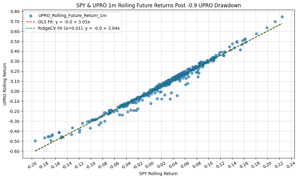
OLS Regression Results
=========================================================================================
Dep. Variable: UPRO_Rolling_Future_Return_1m R-squared: 0.977
Model: OLS Adj. R-squared: 0.977
Method: Least Squares F-statistic: 2.044e+04
Date: Mon, 23 Mar 2026 Prob (F-statistic): 0.00
Time: 22:04:58 Log-Likelihood: 1031.5
No. Observations: 491 AIC: -2059.
Df Residuals: 489 BIC: -2051.
Df Model: 1
Covariance Type: nonrobust
================================================================================================
coef std err t P>|t| [0.025 0.975]
------------------------------------------------------------------------------------------------
const -0.0072 0.001 -5.067 0.000 -0.010 -0.004
SPY_Rolling_Future_Return_1m 3.0532 0.021 142.970 0.000 3.011 3.095
==============================================================================
Omnibus: 245.913 Durbin-Watson: 0.321
Prob(Omnibus): 0.000 Jarque-Bera (JB): 2033.870
Skew: -2.014 Prob(JB): 0.00
Kurtosis: 12.121 Cond. No. 16.0
==============================================================================
Notes:
[1] Standard Errors assume that the covariance matrix of the errors is correctly specified.
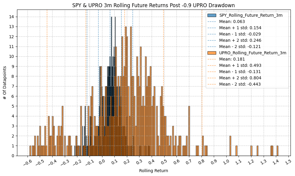
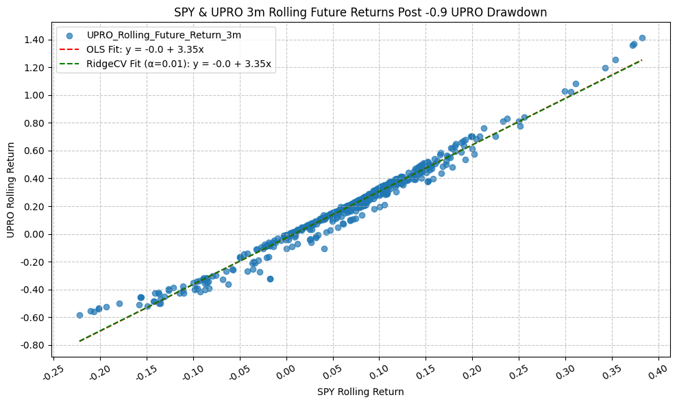
OLS Regression Results
=========================================================================================
Dep. Variable: UPRO_Rolling_Future_Return_3m R-squared: 0.976
Model: OLS Adj. R-squared: 0.976
Method: Least Squares F-statistic: 1.997e+04
Date: Mon, 23 Mar 2026 Prob (F-statistic): 0.00
Time: 22:05:00 Log-Likelihood: 792.83
No. Observations: 491 AIC: -1582.
Df Residuals: 489 BIC: -1573.
Df Model: 1
Covariance Type: nonrobust
================================================================================================
coef std err t P>|t| [0.025 0.975]
------------------------------------------------------------------------------------------------
const -0.0292 0.003 -11.068 0.000 -0.034 -0.024
SPY_Rolling_Future_Return_3m 3.3540 0.024 141.332 0.000 3.307 3.401
==============================================================================
Omnibus: 75.475 Durbin-Watson: 0.347
Prob(Omnibus): 0.000 Jarque-Bera (JB): 481.986
Skew: -0.456 Prob(JB): 2.18e-105
Kurtosis: 7.767 Cond. No. 10.9
==============================================================================
Notes:
[1] Standard Errors assume that the covariance matrix of the errors is correctly specified.
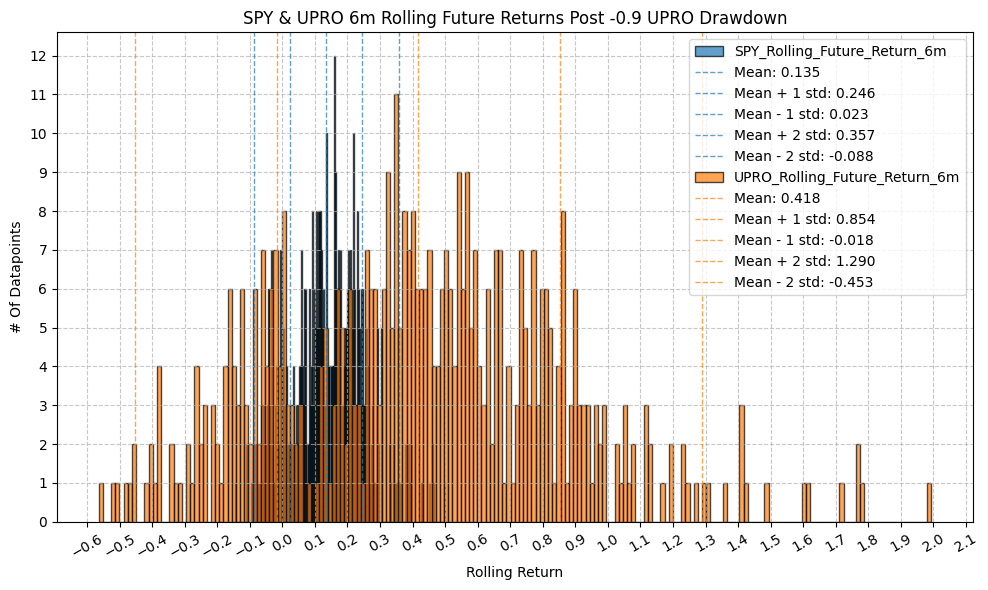
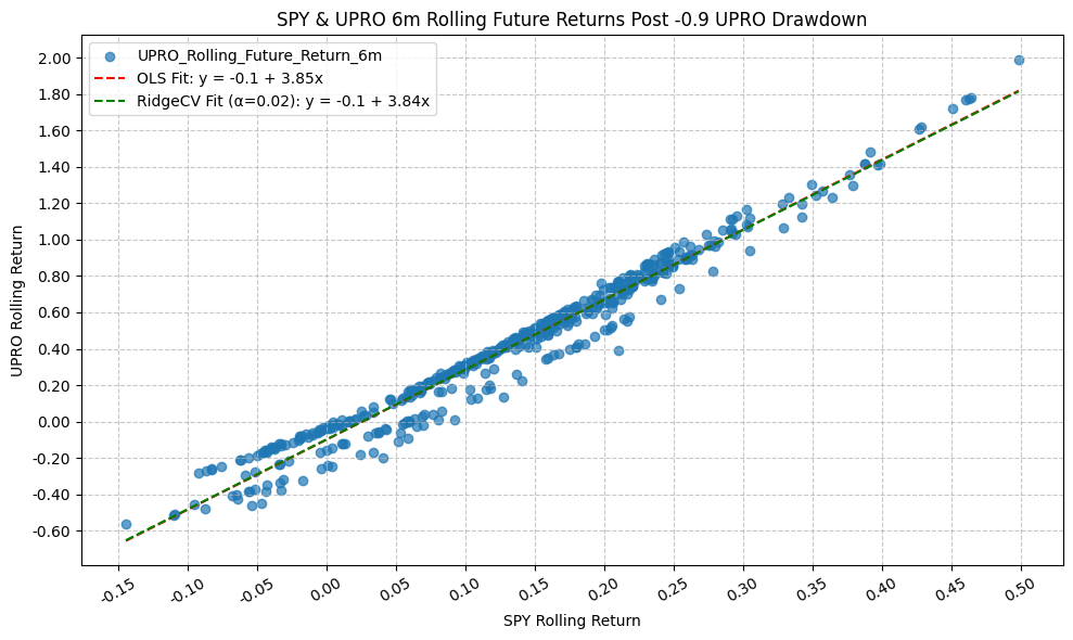
OLS Regression Results
=========================================================================================
Dep. Variable: UPRO_Rolling_Future_Return_6m R-squared: 0.968
Model: OLS Adj. R-squared: 0.968
Method: Least Squares F-statistic: 1.482e+04
Date: Mon, 23 Mar 2026 Prob (F-statistic): 0.00
Time: 22:05:02 Log-Likelihood: 557.06
No. Observations: 491 AIC: -1110.
Df Residuals: 489 BIC: -1102.
Df Model: 1
Covariance Type: nonrobust
================================================================================================
coef std err t P>|t| [0.025 0.975]
------------------------------------------------------------------------------------------------
const -0.0999 0.006 -18.095 0.000 -0.111 -0.089
SPY_Rolling_Future_Return_6m 3.8493 0.032 121.719 0.000 3.787 3.911
==============================================================================
Omnibus: 90.171 Durbin-Watson: 0.148
Prob(Omnibus): 0.000 Jarque-Bera (JB): 142.832
Skew: -1.152 Prob(JB): 9.65e-32
Kurtosis: 4.292 Cond. No. 9.15
==============================================================================
Notes:
[1] Standard Errors assume that the covariance matrix of the errors is correctly specified.
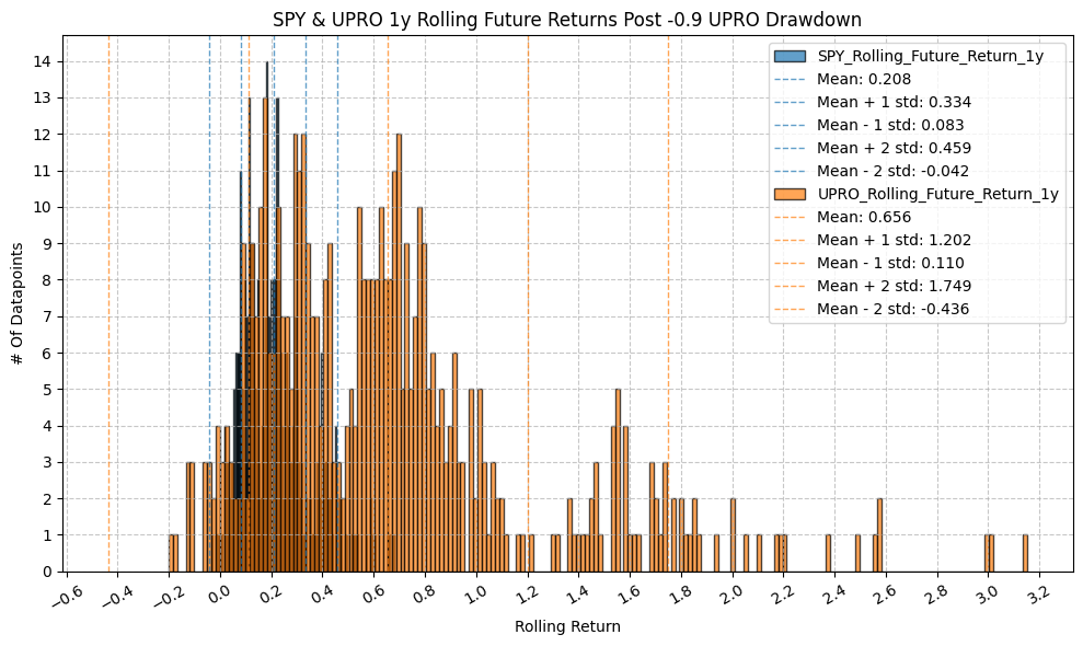
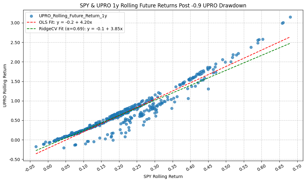
OLS Regression Results
=========================================================================================
Dep. Variable: UPRO_Rolling_Future_Return_1y R-squared: 0.926
Model: OLS Adj. R-squared: 0.926
Method: Least Squares F-statistic: 6140.
Date: Mon, 23 Mar 2026 Prob (F-statistic): 5.83e-279
Time: 22:05:03 Log-Likelihood: 240.67
No. Observations: 491 AIC: -477.3
Df Residuals: 489 BIC: -469.0
Df Model: 1
Covariance Type: nonrobust
================================================================================================
coef std err t P>|t| [0.025 0.975]
------------------------------------------------------------------------------------------------
const -0.2184 0.013 -16.774 0.000 -0.244 -0.193
SPY_Rolling_Future_Return_1y 4.1972 0.054 78.358 0.000 4.092 4.302
==============================================================================
Omnibus: 128.802 Durbin-Watson: 0.094
Prob(Omnibus): 0.000 Jarque-Bera (JB): 299.079
Skew: -1.348 Prob(JB): 1.14e-65
Kurtosis: 5.711 Cond. No. 8.34
==============================================================================
Notes:
[1] Standard Errors assume that the covariance matrix of the errors is correctly specified.
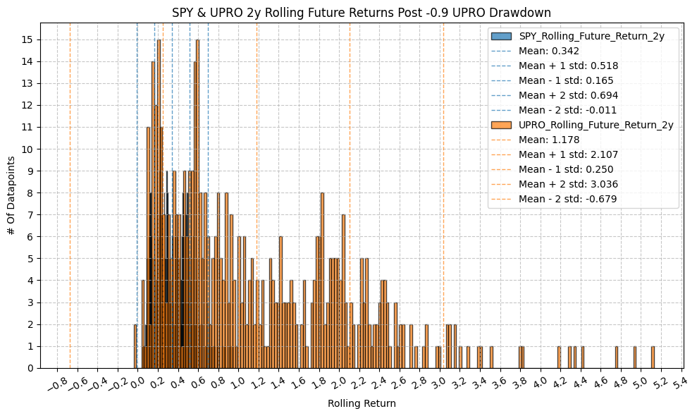
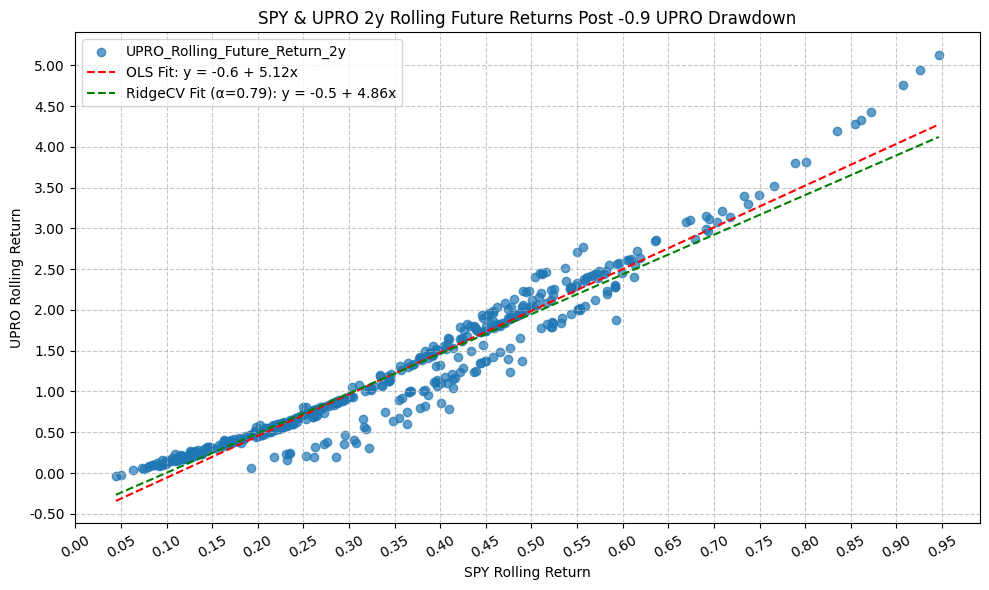
OLS Regression Results
=========================================================================================
Dep. Variable: UPRO_Rolling_Future_Return_2y R-squared: 0.943
Model: OLS Adj. R-squared: 0.943
Method: Least Squares F-statistic: 8061.
Date: Mon, 23 Mar 2026 Prob (F-statistic): 5.45e-306
Time: 22:05:05 Log-Likelihood: 42.554
No. Observations: 491 AIC: -81.11
Df Residuals: 489 BIC: -72.71
Df Model: 1
Covariance Type: nonrobust
================================================================================================
coef std err t P>|t| [0.025 0.975]
------------------------------------------------------------------------------------------------
const -0.5701 0.022 -26.024 0.000 -0.613 -0.527
SPY_Rolling_Future_Return_2y 5.1178 0.057 89.785 0.000 5.006 5.230
==============================================================================
Omnibus: 62.351 Durbin-Watson: 0.075
Prob(Omnibus): 0.000 Jarque-Bera (JB): 116.151
Skew: -0.750 Prob(JB): 6.00e-26
Kurtosis: 4.851 Cond. No. 6.36
==============================================================================
Notes:
[1] Standard Errors assume that the covariance matrix of the errors is correctly specified.
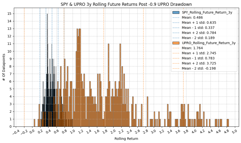
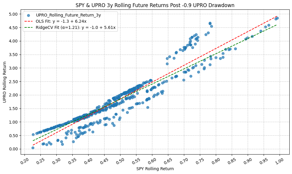
OLS Regression Results
=========================================================================================
Dep. Variable: UPRO_Rolling_Future_Return_3y R-squared: 0.895
Model: OLS Adj. R-squared: 0.894
Method: Least Squares F-statistic: 4155.
Date: Mon, 23 Mar 2026 Prob (F-statistic): 3.74e-241
Time: 22:05:06 Log-Likelihood: -134.10
No. Observations: 491 AIC: 272.2
Df Residuals: 489 BIC: 280.6
Df Model: 1
Covariance Type: nonrobust
================================================================================================
coef std err t P>|t| [0.025 0.975]
------------------------------------------------------------------------------------------------
const -1.2674 0.049 -25.774 0.000 -1.364 -1.171
SPY_Rolling_Future_Return_3y 6.2351 0.097 64.456 0.000 6.045 6.425
==============================================================================
Omnibus: 10.263 Durbin-Watson: 0.052
Prob(Omnibus): 0.006 Jarque-Bera (JB): 14.154
Skew: 0.184 Prob(JB): 0.000844
Kurtosis: 3.746 Cond. No. 8.35
==============================================================================
Notes:
[1] Standard Errors assume that the covariance matrix of the errors is correctly specified.
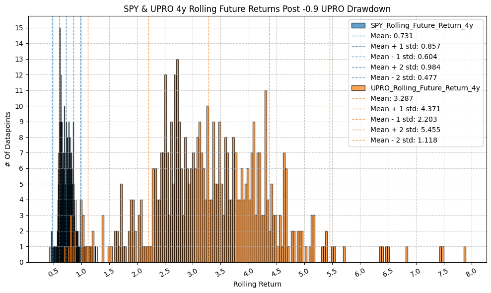
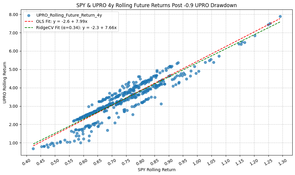
OLS Regression Results
=========================================================================================
Dep. Variable: UPRO_Rolling_Future_Return_4y R-squared: 0.874
Model: OLS Adj. R-squared: 0.874
Method: Least Squares F-statistic: 3400.
Date: Mon, 23 Mar 2026 Prob (F-statistic): 2.56e-222
Time: 22:05:08 Log-Likelihood: -226.80
No. Observations: 491 AIC: 457.6
Df Residuals: 489 BIC: 466.0
Df Model: 1
Covariance Type: nonrobust
================================================================================================
coef std err t P>|t| [0.025 0.975]
------------------------------------------------------------------------------------------------
const -2.5542 0.102 -25.124 0.000 -2.754 -2.354
SPY_Rolling_Future_Return_4y 7.9944 0.137 58.309 0.000 7.725 8.264
==============================================================================
Omnibus: 34.991 Durbin-Watson: 0.062
Prob(Omnibus): 0.000 Jarque-Bera (JB): 40.573
Skew: -0.693 Prob(JB): 1.55e-09
Kurtosis: 3.253 Cond. No. 12.2
==============================================================================
Notes:
[1] Standard Errors assume that the covariance matrix of the errors is correctly specified.
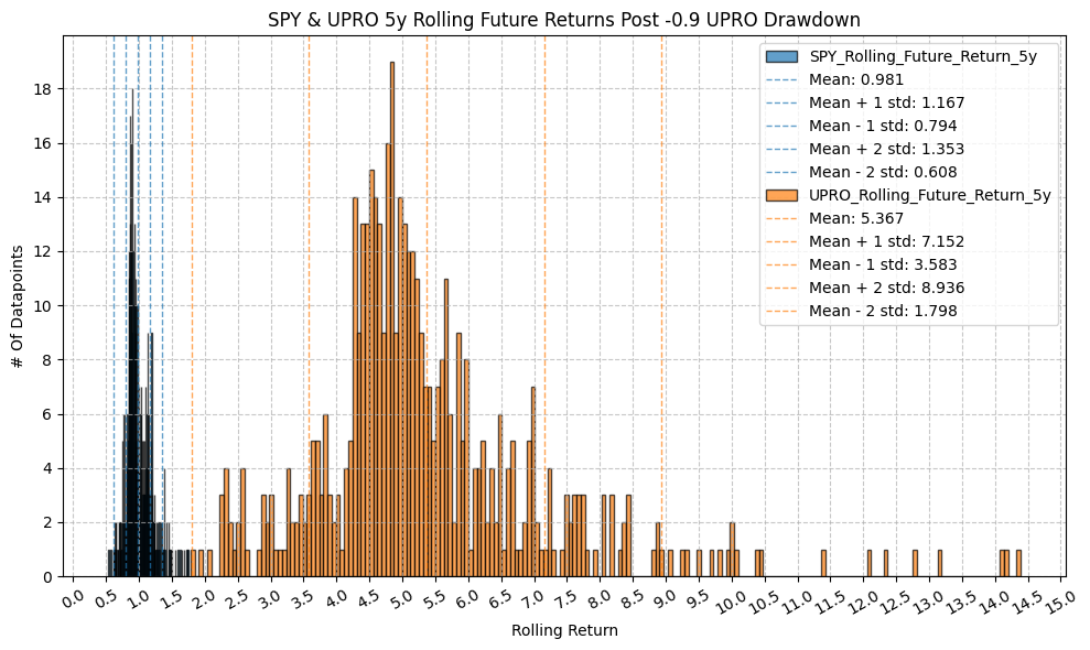
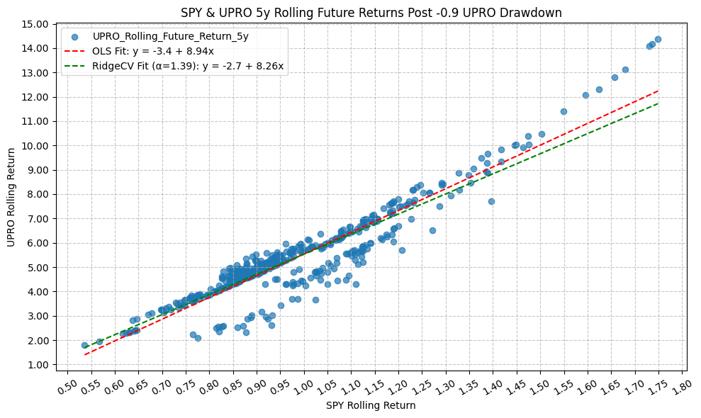
OLS Regression Results
=========================================================================================
Dep. Variable: UPRO_Rolling_Future_Return_5y R-squared: 0.870
Model: OLS Adj. R-squared: 0.870
Method: Least Squares F-statistic: 3285.
Date: Mon, 23 Mar 2026 Prob (F-statistic): 3.96e-219
Time: 22:05:10 Log-Likelihood: -478.85
No. Observations: 491 AIC: 961.7
Df Residuals: 489 BIC: 970.1
Df Model: 1
Covariance Type: nonrobust
================================================================================================
coef std err t P>|t| [0.025 0.975]
------------------------------------------------------------------------------------------------
const -3.3998 0.156 -21.837 0.000 -3.706 -3.094
SPY_Rolling_Future_Return_5y 8.9407 0.156 57.314 0.000 8.634 9.247
==============================================================================
Omnibus: 107.012 Durbin-Watson: 0.059
Prob(Omnibus): 0.000 Jarque-Bera (JB): 209.241
Skew: -1.203 Prob(JB): 3.66e-46
Kurtosis: 5.106 Cond. No. 10.6
==============================================================================
Notes:
[1] Standard Errors assume that the covariance matrix of the errors is correctly specified.
Rolling Returns Following Drawdowns Deviation (SPY & UPRO) #
rolling_returns_positive_future_returns = pd.DataFrame(index=rolling_windows.keys(), data=rolling_windows.values())
rolling_returns_positive_future_returns.reset_index(inplace=True)
rolling_returns_positive_future_returns.rename(columns={"index":"Period", 0:"Days"}, inplace=True)
for drawdown in drawdown_levels:
temp = rolling_returns_drawdown_stats.loc[rolling_returns_drawdown_stats["Drawdown"] == drawdown]
temp = temp[["Period", "Positive_Future_Percentage"]]
temp.rename(columns={"Positive_Future_Percentage" : f"Positive_Future_Percentage_Post_{drawdown}_Drawdown"}, inplace=True)
rolling_returns_positive_future_returns = pd.merge(rolling_returns_positive_future_returns, temp, left_on="Period", right_on="Period", how="outer")
rolling_returns_positive_future_returns.sort_values(by="Days", ascending=True, inplace=True)
rolling_returns_positive_future_returns.drop(columns={"Days"}, inplace=True)
rolling_returns_positive_future_returns.reset_index(drop=True, inplace=True)
pandas_set_decimal_places(2)
display(rolling_returns_positive_future_returns.set_index("Period"))
| Positive_Future_Percentage_Post_-0.1_Drawdown | Positive_Future_Percentage_Post_-0.2_Drawdown | Positive_Future_Percentage_Post_-0.3_Drawdown | Positive_Future_Percentage_Post_-0.4_Drawdown | Positive_Future_Percentage_Post_-0.5_Drawdown | Positive_Future_Percentage_Post_-0.6_Drawdown | Positive_Future_Percentage_Post_-0.7_Drawdown | Positive_Future_Percentage_Post_-0.8_Drawdown | Positive_Future_Percentage_Post_-0.9_Drawdown | |
|---|---|---|---|---|---|---|---|---|---|
| Period | |||||||||
| 1d | 0.54 | 0.54 | 0.54 | 0.54 | 0.54 | 0.55 | 0.55 | 0.55 | 0.55 |
| 1w | 0.57 | 0.57 | 0.56 | 0.56 | 0.56 | 0.56 | 0.57 | 0.57 | 0.59 |
| 1m | 0.63 | 0.61 | 0.61 | 0.61 | 0.62 | 0.62 | 0.62 | 0.65 | 0.68 |
| 3m | 0.67 | 0.65 | 0.63 | 0.63 | 0.65 | 0.65 | 0.66 | 0.68 | 0.77 |
| 6m | 0.70 | 0.69 | 0.68 | 0.67 | 0.69 | 0.70 | 0.73 | 0.75 | 0.79 |
| 1y | 0.73 | 0.73 | 0.73 | 0.72 | 0.74 | 0.79 | 0.84 | 0.87 | 0.96 |
| 2y | 0.77 | 0.78 | 0.78 | 0.78 | 0.77 | 0.81 | 0.92 | 0.99 | 1.00 |
| 3y | 0.72 | 0.72 | 0.72 | 0.72 | 0.72 | 0.74 | 0.87 | 0.99 | 1.00 |
| 4y | 0.69 | 0.69 | 0.68 | 0.68 | 0.68 | 0.71 | 0.81 | 1.00 | 1.00 |
| 5y | 0.66 | 0.66 | 0.66 | 0.66 | 0.65 | 0.67 | 0.74 | 0.97 | 1.00 |
plot_scatter(
df=rolling_returns_positive_future_returns,
x_plot_column="Period",
y_plot_columns=[col for col in rolling_returns_positive_future_returns.columns if col != "Period"],
title="UPRO Future Return by Time Period Post Drawdown",
x_label="Rolling Return Time Period",
x_format="String",
x_format_decimal_places=0,
x_tick_spacing=1,
x_tick_rotation=0,
y_label="Positive Future Return Percentage",
y_format="Decimal",
y_format_decimal_places=2,
y_tick_spacing="Auto",
y_tick_rotation=0,
plot_OLS_regression_line=False,
OLS_column=None,
plot_Ridge_regression_line=False,
Ridge_column=None,
plot_RidgeCV_regression_line=False,
RidgeCV_column=None,
regression_constant=False,
grid=True,
legend=True,
export_plot=False,
plot_file_name=None,
)
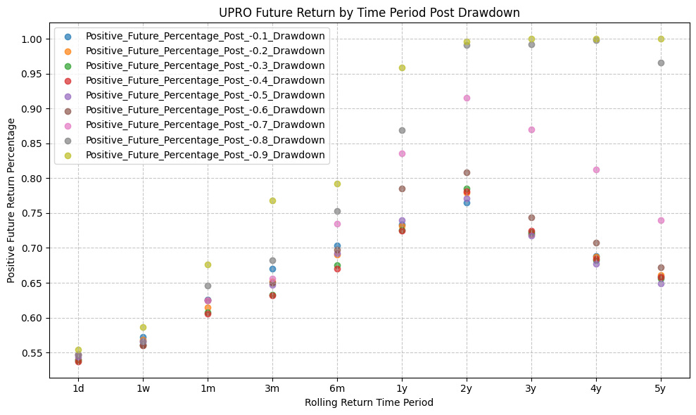
This plot summarizes the future rolling returns well. Similar as to QQQ/TQQQ, for rolling returns up to ~3 months following all drawdown levels, we see the rolling returns of UPRO are positive ~65% of the time.
As we extend the time horizon, out to the 2y, 3y, 4y, and 5y mark, the percentage of positive rolling returns following an 80% drawdown increases significantly, and is greater than 95%. This suggests that while the volatility decay effect is present for UPRO, it may not be as severe as that of TQQQ, which could be due to the less extreme return profile of SPY compared to QQQ.
As an investor, this suggests that the optimal time to buy UPRO would be following a drawdown of 50% or more, and holding for at least 2 years. One could dollar cost average into UPRO following a drawdown of 50% or more, and continue to add to the position with a consistent contribution schedule until all capital has been allocated.
Future Investigation #
There are a couple of ideas for future investigation that would be interesting to explore:
- Expand the analysis of SPY/UPRO to SPX/UPRO (using Bloomberg data for SPX), and extrapolate UPRO return data back to January of 1975.
- Implement and backtest a strategy that DCA’s into UPRO on a consistent schdule (monthly, quarterly, etc.)
Code #
The Jupyter notebook with the functions and all other code is available here.The HTML export of the jupyter notebook is available here.
The PDF export of the jupyter notebook is available here.