Performance Of Various Asset Classes During Fed Policy Cycles

Table of Contents

Introduction #

In this post, we will look into the Fed Funds cycles and evaluate asset class performance during tightening and easing of monetary policy. We’ll pull data for stocks, bonds (IG and HY), and gold, and analyze their returns during different phases of the Fed Funds cycle. We’ll also establish a simple strategy and allocate capital to a specific asset based on the current phase of the cycle, and evaluate the performance of this strategy over time.

Python Imports #

# Standard Library
import datetime
import os
import sys
import warnings

from datetime import datetime
from pathlib import Path

# Data Handling
import numpy as np
import pandas as pd

# Data Sources
import pandas_datareader.data as web

# Statistical Analysis
import statsmodels.api as sm

# Suppress warnings
warnings.filterwarnings("ignore")

# Add the source subdirectory to the system path to allow import config from settings.py
current_directory = Path(os.getcwd())
website_base_directory = current_directory.parent.parent.parent
src_directory = website_base_directory / "src"
sys.path.append(str(src_directory)) if str(src_directory) not in sys.path else None

# Import settings.py
from settings import config

# Add configured directories from config to path
SOURCE_DIR = config("SOURCE_DIR")
sys.path.append(str(Path(SOURCE_DIR))) if str(Path(SOURCE_DIR)) not in sys.path else None

# Add other configured directories
BASE_DIR = config("BASE_DIR")
CONTENT_DIR = config("CONTENT_DIR")
POSTS_DIR = config("POSTS_DIR")
PAGES_DIR = config("PAGES_DIR")
PUBLIC_DIR = config("PUBLIC_DIR")
SOURCE_DIR = config("SOURCE_DIR")
DATA_DIR = config("DATA_DIR")
DATA_MANUAL_DIR = config("DATA_MANUAL_DIR")

Python Functions #

Here are the functions needed for this project:

bb_clean_data: Takes an Excel export from Bloomberg, removes the miscellaneous headings/rows, and returns a DataFrame.
calc_fed_cycle_asset_performance: Calculates metrics for an asset based on a specified Fed tightening/easing cycle.
load_data: Load data from a CSV, Excel, or Pickle file into a pandas DataFrame.
pandas_set_decimal_places: Set the number of decimal places displayed for floating-point numbers in pandas.
plot_bar_returns_ffr_change: Plot the bar chart of the cumulative or annualized returns for the asset class along with the change in the Fed Funds Rate.
plot_scatter_regression_ffr_vs_returns: Plot the scatter plot and regression of the annualized return for the asset class along with the annualized change in the Fed Funds Rate.
plot_time_series: Plot the time series data from a DataFrame for a specified date range and columns.
summary_stats: Generate summary statistics for a series of returns.

from bb_clean_data import bb_clean_data
from calc_fed_cycle_asset_performance import calc_fed_cycle_asset_performance
from load_data import load_data
from pandas_set_decimal_places import pandas_set_decimal_places
from plot_bar_returns_ffr_change import plot_bar_returns_ffr_change
from plot_scatter_regression_ffr_vs_returns import plot_scatter_regression_ffr_vs_returns
from plot_time_series import plot_time_series
from summary_stats import summary_stats

Data Overview #

Acquire & Plot Fed Funds Data #

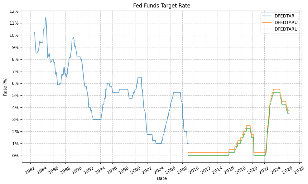
First, let’s get the data for the Fed Funds target rate (FFR). This data is found in 3 different datasets from FRED.

# Set decimal places
pandas_set_decimal_places(4)

# Pull Federal Funds Target Rate (DISCONTINUED) (DFEDTAR)
fedfunds_target_old = web.DataReader("DFEDTAR", "fred", start="1900-01-01", end=datetime.today())

# Pull Federal Funds Target Range - Upper Limit (DFEDTARU)
fedfunds_target_new_upper = web.DataReader("DFEDTARU", "fred", start="1900-01-01", end=datetime.today())

# Pull Federal Funds Target Range - Lower Limit (DFEDTARL)
fedfunds_target_new_lower = web.DataReader("DFEDTARL", "fred", start="1900-01-01", end=datetime.today())

# Merge the datasets together
fedfunds_combined = pd.concat([fedfunds_target_old, fedfunds_target_new_upper, fedfunds_target_new_lower], axis=1)

# Divide all values by 100 to get decimal rates
for col in fedfunds_combined.columns:
    fedfunds_combined[col] = fedfunds_combined[col] / 100

# Resample to month-end (as if we know the rate at the end of the month)
fedfunds_monthly = fedfunds_combined.resample("ME").last()

display(fedfunds_monthly)

	DFEDTAR	DFEDTARU	DFEDTARL
DATE
1982-09-30	0.1025	NaN	NaN
1982-10-31	0.0950	NaN	NaN
1982-11-30	0.0900	NaN	NaN
1982-12-31	0.0850	NaN	NaN
1983-01-31	0.0850	NaN	NaN
...	...	...	...
2025-11-30	NaN	0.0400	0.0375
2025-12-31	NaN	0.0375	0.0350
2026-01-31	NaN	0.0375	0.0350
2026-02-28	NaN	0.0375	0.0350
2026-03-31	NaN	0.0375	0.0350

523 rows × 3 columns

We can then generate several useful plots. First, the Fed Funds target rate:

plot_time_series(
    df=fedfunds_monthly,
    plot_start_date=None,
    plot_end_date=None,
    plot_columns=["DFEDTAR", "DFEDTARU", "DFEDTARL"],
    title="Fed Funds Target Rate",
    x_label="Date",
    x_format="Year",
    x_tick_spacing=2,
    x_tick_rotation=30,
    y_label="Rate (%)",
    y_format="Percentage",
    y_format_decimal_places=0,
    y_tick_spacing=0.01,
    y_tick_rotation=0,
    grid=True,
    legend=True,
    export_plot=False,
    plot_file_name=None,
)

png

# First drop the lower column and merge
fedfunds_monthly["fed_funds"] = fedfunds_monthly["DFEDTAR"].combine_first(fedfunds_monthly["DFEDTARU"])
fedfunds_monthly = fedfunds_monthly.drop(columns=["DFEDTARL", "DFEDTARU", "DFEDTAR"])

# Compute change in rate from either column
fedfunds_monthly["fed_funds_change"] = fedfunds_monthly["fed_funds"].diff()

display(fedfunds_monthly)

	fed_funds	fed_funds_change
DATE
1982-09-30	0.1025	NaN
1982-10-31	0.0950	-0.0075
1982-11-30	0.0900	-0.0050
1982-12-31	0.0850	-0.0050
1983-01-31	0.0850	0.0000
...	...	...
2025-11-30	0.0400	0.0000
2025-12-31	0.0375	-0.0025
2026-01-31	0.0375	0.0000
2026-02-28	0.0375	0.0000
2026-03-31	0.0375	0.0000

523 rows × 2 columns

And then the change in FFR from month-to-month:

plot_time_series(
    df=fedfunds_monthly,
    plot_start_date=None,
    plot_end_date=None,
    plot_columns=["fed_funds_change"],
    title="Fed Funds Change In Rate",
    x_label="Date",
    x_format="Year",
    x_tick_spacing=2,
    x_tick_rotation=30,
    y_label="Rate Change (%)",
    y_format="Percentage",
    y_format_decimal_places=2,
    y_tick_spacing=0.0025,
    y_tick_rotation=0,
    grid=True,
    legend=False,
    export_plot=False,
    plot_file_name=None,
)

png

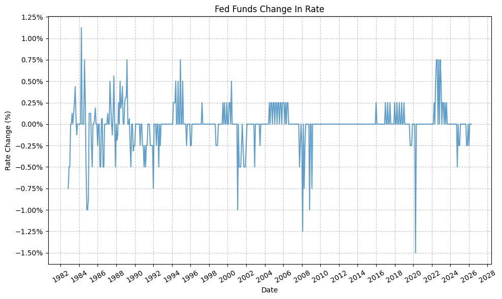
This plot, in particular, makes it easy to show the monthly increase and decrease in the FFR, as well as the magnitude of the change (i.e. slow, drawn-out increases or decreases or abrupt large increases or decreases).

Define Fed Policy Cycles #

Next, we will define the Fed policy tightening and easing cycles:

# Set timeframe
start_date = "1989-12-15"
end_date = "2026-01-31"

# Copy DataFrame to avoid modifying original
fedfunds_cycles = fedfunds_monthly.copy()
fedfunds_cycles = fedfunds_cycles.loc[start_date:end_date]

# Reset index
fedfunds_cycles = fedfunds_cycles.reset_index()

# Drop the "fed_funds_change" column as we will use it to determine the cycle type later, but we don't need it in the final dataframe
fedfunds_cycles = fedfunds_cycles.drop(columns=["fed_funds_change"])

# Rename the date column to "Start Date", and the "fed_funds" column to "Fed Funds Start"
fedfunds_cycles = fedfunds_cycles.rename(columns={"DATE": "start_date", "fed_funds": "fed_funds_start"})

# Copy the "Start Date" column to a new column called "End Date" and shift it up by one row
fedfunds_cycles["end_date"] = fedfunds_cycles["start_date"].shift(-1)

# Copy the "Fed Funds Start" column to a new column called "Fed Funds End" and shift it up by one row
fedfunds_cycles["fed_funds_end"] = fedfunds_cycles["fed_funds_start"].shift(-1)

# Calculate the change in Fed Funds rate for each cycle
fedfunds_cycles["fed_funds_change"] = fedfunds_cycles["fed_funds_end"] - fedfunds_cycles["fed_funds_start"]

# Based on "Fed Funds Change" column, determine if the rate is increasing, decreasing, or unchanged
fedfunds_cycles["cycle"] = fedfunds_cycles["fed_funds_change"].apply(
    lambda x: "Tightening" if x > 0 else ("Easing" if x < 0 else "Neutral"))

display(fedfunds_cycles)

	start_date	fed_funds_start	end_date	fed_funds_end	fed_funds_change	cycle
0	1989-12-31	0.0825	1990-01-31	0.0825	0.0000	Neutral
1	1990-01-31	0.0825	1990-02-28	0.0825	0.0000	Neutral
2	1990-02-28	0.0825	1990-03-31	0.0825	0.0000	Neutral
3	1990-03-31	0.0825	1990-04-30	0.0825	0.0000	Neutral
4	1990-04-30	0.0825	1990-05-31	0.0825	0.0000	Neutral
...	...	...	...	...	...	...
429	2025-09-30	0.0425	2025-10-31	0.0400	-0.0025	Easing
430	2025-10-31	0.0400	2025-11-30	0.0400	0.0000	Neutral
431	2025-11-30	0.0400	2025-12-31	0.0375	-0.0025	Easing
432	2025-12-31	0.0375	2026-01-31	0.0375	0.0000	Neutral
433	2026-01-31	0.0375	NaT	NaN	NaN	Neutral

434 rows × 6 columns

Grouping the consecutive months of tightening and easing together, we can create a DataFrame that gives us the cumulative change in the FFR for each cycle, as well as the start and end dates for each cycle. This will be useful for evaluating asset class performance during these cycles.

fedfunds_grouped_cycles = fedfunds_cycles.copy()

# Create a group key that increments whenever the Cycle value changes
fedfunds_grouped_cycles['group'] = (fedfunds_grouped_cycles['cycle'] != fedfunds_grouped_cycles['cycle'].shift(1)).cumsum()

# Group by both the group key and Cycle label
cycle_ranges = (
    fedfunds_grouped_cycles.groupby(['group', 'cycle'], sort=False)
    .agg(
        start_date=('start_date', 'first'),
        end_date=('end_date', 'last'),
        fed_funds_start=('fed_funds_start', 'first'),
        fed_funds_end=('fed_funds_end', 'last')
    )
    .reset_index(drop=False)
    .drop(columns='group')
)

display(cycle_ranges)

	cycle	start_date	end_date	fed_funds_start	fed_funds_end
0	Neutral	1989-12-31	1990-06-30	0.0825	0.0825
1	Easing	1990-06-30	1990-07-31	0.0825	0.0800
2	Neutral	1990-07-31	1990-09-30	0.0800	0.0800
3	Easing	1990-09-30	1991-04-30	0.0800	0.0575
4	Neutral	1991-04-30	1991-07-31	0.0575	0.0575
...	...	...	...	...	...
116	Neutral	2024-12-31	2025-08-31	0.0450	0.0450
117	Easing	2025-08-31	2025-10-31	0.0450	0.0400
118	Neutral	2025-10-31	2025-11-30	0.0400	0.0400
119	Easing	2025-11-30	2025-12-31	0.0400	0.0375
120	Neutral	2025-12-31	2026-01-31	0.0375	0.0375

121 rows × 5 columns

Furthermore, we will make the assumption that any “Neutral” months (i.e. months where the FFR did not change) are part of the preceding cycle – to a point. For example, if we have a tightening month followed by a neutral month, we will consider the neutral month to be part of the tightening cycle. This is a simplifying assumption, but it allows us to categorize all months into either tightening or easing cycles without having to create a separate category for neutral months. From a practical standpoint, this also makes it easier to evaluate asset class performance during these cycles, as we can simply look at the performance during the tightening and easing cycles without having to worry about the neutral months. We will foward fill no more than 6 months of neutral months, however, as it would be unreasonable to assume that a month of neutral policy is part of the preceding cycle if it has been 6 months since the last change in policy.

fedfunds_grouped_cycles = fedfunds_cycles.copy()

# Forward fill cycle labels preceding "Neutral" cycles
fedfunds_grouped_cycles['cycle_filled'] = fedfunds_grouped_cycles['cycle'].replace('Neutral', pd.NA).ffill(limit=6)

# Replaced any remaining <NA> values with "Modified Tightening"
fedfunds_grouped_cycles['cycle_filled'] = fedfunds_grouped_cycles['cycle_filled'].fillna('Modified Tightening')

# Create a group key that increments whenever the Cycle value changes
fedfunds_grouped_cycles['group'] = (fedfunds_grouped_cycles['cycle_filled'] != fedfunds_grouped_cycles['cycle_filled'].shift(1)).cumsum()

# Group by both the group key and Cycle label
cycle_ranges = (
    fedfunds_grouped_cycles.groupby(['group', 'cycle_filled'], sort=False)
    .agg(
        start_date=('start_date', 'first'),
        end_date=('end_date', 'last'),
        fed_funds_start=('fed_funds_start', 'first'),
        fed_funds_end=('fed_funds_end', 'last')
    )
    .reset_index(drop=False)
    .drop(columns='group')
)

# Calc change in Fed Funds rate for each cycle
cycle_ranges["fed_funds_change"] = cycle_ranges["fed_funds_end"] - cycle_ranges["fed_funds_start"]

# Add cycle labels
cycle_labels = [f"Cycle {i+1}" for i in range(len(cycle_ranges))]

# Combine labels with cycle_ranges
cycle_ranges['cycle_label'] = cycle_labels

display(cycle_ranges)

	cycle_filled	start_date	end_date	fed_funds_start	fed_funds_end	fed_funds_change	cycle_label
0	Modified Tightening	1989-12-31	1990-06-30	0.0825	0.0825	0.0000	Cycle 1
1	Easing	1990-06-30	1993-03-31	0.0825	0.0300	-0.0525	Cycle 2
2	Modified Tightening	1993-03-31	1994-01-31	0.0300	0.0300	0.0000	Cycle 3
3	Tightening	1994-01-31	1995-06-30	0.0300	0.0600	0.0300	Cycle 4
4	Easing	1995-06-30	1996-07-31	0.0600	0.0525	-0.0075	Cycle 5
5	Modified Tightening	1996-07-31	1997-02-28	0.0525	0.0525	0.0000	Cycle 6
6	Tightening	1997-02-28	1997-09-30	0.0525	0.0550	0.0025	Cycle 7
7	Modified Tightening	1997-09-30	1998-08-31	0.0550	0.0550	0.0000	Cycle 8
8	Easing	1998-08-31	1999-05-31	0.0550	0.0475	-0.0075	Cycle 9
9	Tightening	1999-05-31	2000-11-30	0.0475	0.0650	0.0175	Cycle 10
10	Modified Tightening	2000-11-30	2000-12-31	0.0650	0.0650	0.0000	Cycle 11
11	Easing	2000-12-31	2002-06-30	0.0650	0.0175	-0.0475	Cycle 12
12	Modified Tightening	2002-06-30	2002-10-31	0.0175	0.0175	0.0000	Cycle 13
13	Easing	2002-10-31	2003-12-31	0.0175	0.0100	-0.0075	Cycle 14
14	Modified Tightening	2003-12-31	2004-05-31	0.0100	0.0100	0.0000	Cycle 15
15	Tightening	2004-05-31	2006-12-31	0.0100	0.0525	0.0425	Cycle 16
16	Modified Tightening	2006-12-31	2007-08-31	0.0525	0.0525	0.0000	Cycle 17
17	Easing	2007-08-31	2009-07-31	0.0525	0.0025	-0.0500	Cycle 18
18	Modified Tightening	2009-07-31	2015-11-30	0.0025	0.0025	0.0000	Cycle 19
19	Tightening	2015-11-30	2016-06-30	0.0025	0.0050	0.0025	Cycle 20
20	Modified Tightening	2016-06-30	2016-11-30	0.0050	0.0050	0.0000	Cycle 21
21	Tightening	2016-11-30	2019-06-30	0.0050	0.0250	0.0200	Cycle 22
22	Modified Tightening	2019-06-30	2019-07-31	0.0250	0.0250	0.0000	Cycle 23
23	Easing	2019-07-31	2020-09-30	0.0250	0.0025	-0.0225	Cycle 24
24	Modified Tightening	2020-09-30	2022-02-28	0.0025	0.0025	0.0000	Cycle 25
25	Tightening	2022-02-28	2024-01-31	0.0025	0.0550	0.0525	Cycle 26
26	Modified Tightening	2024-01-31	2024-08-31	0.0550	0.0550	0.0000	Cycle 27
27	Easing	2024-08-31	2025-06-30	0.0550	0.0450	-0.0100	Cycle 28
28	Modified Tightening	2025-06-30	2025-08-31	0.0450	0.0450	0.0000	Cycle 29
29	Easing	2025-08-31	2026-01-31	0.0450	0.0375	-0.0075	Cycle 30

Asset Class Performance By Fed Policy Cycle #

Moving on, we will now look at the performance of four (4) different asset classes during each Fed cycle. We’ll use the following Bloomberg indices:

SPXT_S&P 500 Total Return Index (Stocks)
SPBDU10T_S&P US Treasury Bond 7-10 Year Total Return Index (Bonds)
LF98TRUU_Bloomberg US Corporate High Yield Total Return Index Value Unhedged USD (High Yield Bonds)
XAU_Gold USD Spot (Gold)

Stocks #

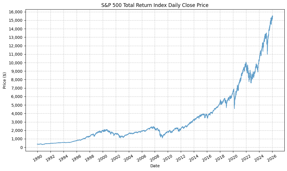
First, we will clean and load the data for the S&P 500 Total Return Index (SPXT):

pandas_set_decimal_places(2)

bb_clean_data(
    base_directory=DATA_DIR,
    fund_ticker_name="SPXT_S&P 500 Total Return Index",
    source="Bloomberg",
    asset_class="Indices",
    excel_export=True,
    pickle_export=True,
    output_confirmation=False,
)

spxt = load_data(
    base_directory=DATA_DIR,
    ticker="SPXT_S&P 500 Total Return Index_Clean",
    source="Bloomberg", 
    asset_class="Indices",
    timeframe="Daily",
    file_format="pickle",
)

# Filter SPXT to date range
spxt = spxt[(spxt.index >= pd.to_datetime(start_date)) & (spxt.index <= pd.to_datetime(end_date))]

# Drop everything except the "close" column
spxt = spxt[["Close"]]

# Resample to monthly frequency
spxt_monthly = spxt.resample("M").last()
spxt_monthly["Monthly_Return"] = spxt_monthly["Close"].pct_change()
spxt_monthly = spxt_monthly.dropna()

display(spxt_monthly)

	Close	Monthly_Return
Date
1990-01-31	353.94	-0.07
1990-02-28	358.50	0.01
1990-03-31	368	0.03
1990-04-30	358.81	-0.02
1990-05-31	393.80	0.10
...	...	...
2025-09-30	14826.80	0.04
2025-10-31	15173.95	0.02
2025-11-30	15211.14	0.00
2025-12-31	15220.45	0.00
2026-01-31	15441.15	0.01

433 rows × 2 columns

Next, we can plot the price history before calculating the cycle performance:

plot_time_series(
    df=spxt,
    plot_start_date=None,
    plot_end_date=None,
    plot_columns=["Close"],
    title="S&P 500 Total Return Index Daily Close Price",
    x_label="Date",
    x_format="Year",
    x_tick_spacing=2,
    x_tick_rotation=30,
    y_label="Price ($)",
    y_format="Decimal",
    y_format_decimal_places=0,
    y_tick_spacing=1000,
    y_tick_rotation=0,
    grid=True,
    legend=False,
    export_plot=False,
    plot_file_name=None,
)

png

Next, we will calculate the performance for SPY based on the pre-defined Fed cycles:

spxt_cycles = calc_fed_cycle_asset_performance(
    start_date=cycle_ranges["start_date"],
    end_date=cycle_ranges["end_date"],
    label=cycle_ranges["cycle_label"],
    fed_funds_change=cycle_ranges["fed_funds_change"],
    monthly_returns=spxt_monthly,
)

display(spxt_cycles)

	Cycle	Start	End	Months	CumulativeReturn	CumulativeReturnPct	AverageMonthlyReturn	AverageMonthlyReturnPct	AnnualizedReturn	AnnualizedReturnPct	Volatility	FedFundsChange	FedFundsChange_bps	FFR_AnnualizedChange	FFR_AnnualizedChange_bps	Label
0	Cycle 1	1989-12-31	1990-06-30	6	0.03	3.09	0.01	0.63	0.06	6.28	0.19	0.00	0.00	0.00	0.00	Cycle 1, 1989-12-31 to 1990-06-30
1	Cycle 2	1990-06-30	1993-03-31	34	0.37	36.80	0.01	1.00	0.12	11.69	0.13	-0.05	-525.00	-0.02	-185.29	Cycle 2, 1990-06-30 to 1993-03-31
2	Cycle 3	1993-03-31	1994-01-31	11	0.11	11.36	0.01	1.00	0.12	12.45	0.07	0.00	0.00	0.00	0.00	Cycle 3, 1993-03-31 to 1994-01-31
3	Cycle 4	1994-01-31	1995-06-30	18	0.22	21.80	0.01	1.14	0.14	14.05	0.10	0.03	300.00	0.02	200.00	Cycle 4, 1994-01-31 to 1995-06-30
4	Cycle 5	1995-06-30	1996-07-31	14	0.23	23.23	0.02	1.53	0.20	19.61	0.08	-0.01	-75.00	-0.01	-64.29	Cycle 5, 1995-06-30 to 1996-07-31
5	Cycle 6	1996-07-31	1997-02-28	8	0.20	19.59	0.02	2.34	0.31	30.78	0.14	0.00	0.00	0.00	0.00	Cycle 6, 1996-07-31 to 1997-02-28
6	Cycle 7	1997-02-28	1997-09-30	8	0.22	22.02	0.03	2.63	0.35	34.78	0.18	0.00	25.00	0.00	37.50	Cycle 7, 1997-02-28 to 1997-09-30
7	Cycle 8	1997-09-30	1998-08-31	12	0.08	8.09	0.01	0.81	0.08	8.09	0.20	0.00	0.00	0.00	0.00	Cycle 8, 1997-09-30 to 1998-08-31
8	Cycle 9	1998-08-31	1999-05-31	10	0.18	17.55	0.02	1.85	0.21	21.42	0.24	-0.01	-75.00	-0.01	-90.00	Cycle 9, 1998-08-31 to 1999-05-31
9	Cycle 10	1999-05-31	2000-11-30	19	0.00	0.40	0.00	0.13	0.00	0.25	0.16	0.02	175.00	0.01	110.53	Cycle 10, 1999-05-31 to 2000-11-30
10	Cycle 11	2000-11-30	2000-12-31	2	-0.07	-7.43	-0.04	-3.70	-0.37	-37.09	0.21	0.00	0.00	0.00	0.00	Cycle 11, 2000-11-30 to 2000-12-31
11	Cycle 12	2000-12-31	2002-06-30	19	-0.23	-23.11	-0.01	-1.25	-0.15	-15.29	0.17	-0.05	-475.00	-0.03	-300.00	Cycle 12, 2000-12-31 to 2002-06-30
12	Cycle 13	2002-06-30	2002-10-31	5	-0.16	-16.41	-0.03	-3.27	-0.35	-34.96	0.28	0.00	0.00	0.00	0.00	Cycle 13, 2002-06-30 to 2002-10-31
13	Cycle 14	2002-10-31	2003-12-31	15	0.40	39.54	0.02	2.33	0.31	30.55	0.14	-0.01	-75.00	-0.01	-60.00	Cycle 14, 2002-10-31 to 2003-12-31
14	Cycle 15	2003-12-31	2004-05-31	6	0.07	6.79	0.01	1.13	0.14	14.04	0.09	0.00	0.00	0.00	0.00	Cycle 15, 2003-12-31 to 2004-05-31
15	Cycle 16	2004-05-31	2006-12-31	32	0.35	34.57	0.01	0.95	0.12	11.78	0.07	0.04	425.00	0.02	159.38	Cycle 16, 2004-05-31 to 2006-12-31
16	Cycle 17	2006-12-31	2007-08-31	9	0.07	6.67	0.01	0.75	0.09	8.99	0.09	0.00	0.00	0.00	0.00	Cycle 17, 2006-12-31 to 2007-08-31
17	Cycle 18	2007-08-31	2009-07-31	24	-0.29	-28.84	-0.01	-1.19	-0.16	-15.64	0.23	-0.05	-500.00	-0.03	-250.00	Cycle 18, 2007-08-31 to 2009-07-31
18	Cycle 19	2009-07-31	2015-11-30	77	1.59	159.04	0.01	1.31	0.16	15.99	0.13	0.00	0.00	0.00	0.00	Cycle 19, 2009-07-31 to 2015-11-30
19	Cycle 20	2015-11-30	2016-06-30	8	0.03	2.50	0.00	0.36	0.04	3.78	0.11	0.00	25.00	0.00	37.50	Cycle 20, 2015-11-30 to 2016-06-30
20	Cycle 21	2016-06-30	2016-11-30	6	0.06	6.01	0.01	1.00	0.12	12.38	0.08	0.00	0.00	0.00	0.00	Cycle 21, 2016-06-30 to 2016-11-30
21	Cycle 22	2016-11-30	2019-06-30	32	0.46	46.03	0.01	1.26	0.15	15.26	0.13	0.02	200.00	0.01	75.00	Cycle 22, 2016-11-30 to 2019-06-30
22	Cycle 23	2019-06-30	2019-07-31	2	0.09	8.59	0.04	4.24	0.64	63.93	0.14	0.00	0.00	0.00	0.00	Cycle 23, 2019-06-30 to 2019-07-31
23	Cycle 24	2019-07-31	2020-09-30	15	0.17	17.10	0.01	1.23	0.13	13.46	0.21	-0.02	-225.00	-0.02	-180.00	Cycle 24, 2019-07-31 to 2020-09-30
24	Cycle 25	2020-09-30	2022-02-28	18	0.28	27.73	0.01	1.46	0.18	17.72	0.15	0.00	0.00	0.00	0.00	Cycle 25, 2020-09-30 to 2022-02-28
25	Cycle 26	2022-02-28	2024-01-31	24	0.11	10.89	0.01	0.58	0.05	5.31	0.19	0.05	525.00	0.03	262.50	Cycle 26, 2022-02-28 to 2024-01-31
26	Cycle 27	2024-01-31	2024-08-31	8	0.20	19.53	0.02	2.29	0.31	30.68	0.10	0.00	0.00	0.00	0.00	Cycle 27, 2024-01-31 to 2024-08-31
27	Cycle 28	2024-08-31	2025-06-30	11	0.14	13.78	0.01	1.24	0.15	15.12	0.13	-0.01	-100.00	-0.01	-109.09	Cycle 28, 2024-08-31 to 2025-06-30
28	Cycle 29	2025-06-30	2025-08-31	3	0.10	9.62	0.03	3.12	0.44	44.41	0.06	0.00	0.00	0.00	0.00	Cycle 29, 2025-06-30 to 2025-08-31
29	Cycle 30	2025-08-31	2026-01-31	6	0.10	10.13	0.02	1.63	0.21	21.29	0.05	-0.01	-75.00	-0.01	-150.00	Cycle 30, 2025-08-31 to 2026-01-31

This gives us the following data points:

Cycle start date
Cycle end date
Number of months in the cycle
Cumulative return during the cycle (decimal and percent)
Average monthly return during the cycle (decimal and percent)
Annualized return during the cycle (decimal and percent)
Return volatility during the cycle
Cumulative change in FFR during the cycle (decimal and basis points)
Annualized change in FFR during the cycle (decimal and basis points)

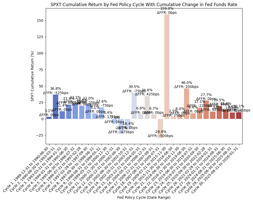
From the above DataFrame, we can then plot the cumulative and annualized returns for each cycle in a bar chart. First, the cumulative returns along with the cumulative change in FFR:

plot_bar_returns_ffr_change(
    cycle_df=spxt_cycles,
    asset_label="SPXT",
    annualized_or_cumulative="Cumulative",
)

png

And then the annualized returns along with the annualized change in FFR:

plot_bar_returns_ffr_change(
    cycle_df=spxt_cycles,
    asset_label="SPXT",
    annualized_or_cumulative="Annualized",
)

png

The cumulative returns plot is not particularly insightful, but there are some interesting observations to be gained from the annualized returns plot. During the past two (2) rate cutting cycles (cycles 11/12/13/14 and 18), stocks have exhibited negative returns during the rate cutting cycle. However, after the rate cutting cycle was complete, returns during the following cycle (when rates were usually flat) were quite strong and higher than the historical mean return for the S&P 500. The economic intuition for this behavior is valid; as the economy weakens, investors are concerned about the pricing of equities, the returns become negative, and the Fed responds with cutting rates. The exact timing of when the Fed begins cutting rates is one of the unknowns; the Fed could be ahead of the curve, cutting rates as economic data begins to prompt that action, or behind the curve, where the ecomony rolls over rapidly and even the Fed’s actions are not enough to halt the economic contraction.

Finally, we can run an OLS regression to check fit:

df = spxt_cycles

#=== Don't modify below this line ===

# Run OLS regression with statsmodels
X = df["FFR_AnnualizedChange_bps"]
y = df["AnnualizedReturnPct"]
X = sm.add_constant(X)
model = sm.OLS(y, X).fit()
print(model.summary())
print(f"Intercept: {model.params[0]}, Slope: {model.params[1]}")  # Intercept and slope

# Calc X and Y values for regression line
X_vals = np.linspace(X.min(), X.max(), 100)
Y_vals = model.params[0] + model.params[1] * X_vals

                             OLS Regression Results                            
===============================================================================
Dep. Variable:     AnnualizedReturnPct   R-squared:                       0.017
Model:                             OLS   Adj. R-squared:                 -0.018
Method:                  Least Squares   F-statistic:                    0.4786
Date:                 Mon, 23 Mar 2026   Prob (F-statistic):              0.495
Time:                         22:08:21   Log-Likelihood:                -132.24
No. Observations:                   30   AIC:                             268.5
Df Residuals:                       28   BIC:                             271.3
Df Model:                            1                                         
Covariance Type:             nonrobust                                         
============================================================================================
                               coef    std err          t      P>|t|      [0.025      0.975]
--------------------------------------------------------------------------------------------
const                       13.0760      3.792      3.448      0.002       5.308      20.844
FFR_AnnualizedChange_bps     0.0221      0.032      0.692      0.495      -0.043       0.087
==============================================================================
Omnibus:                        4.070   Durbin-Watson:                   1.523
Prob(Omnibus):                  0.131   Jarque-Bera (JB):                2.894
Skew:                          -0.320   Prob(JB):                        0.235
Kurtosis:                       4.381   Cond. No.                         120.
==============================================================================

Notes:
[1] Standard Errors assume that the covariance matrix of the errors is correctly specified.
Intercept: 13.076015539043272, Slope: 0.022056651501767076

And then plot the regression line along with the values:

plot_scatter_regression_ffr_vs_returns(
    cycle_df=spxt_cycles,
    asset_label="SPXT",
    x_vals=X_vals,
    y_vals=Y_vals,
    intercept=model.params[0],
    slope=model.params[1],
)

png

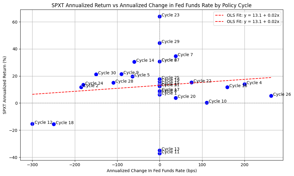
Here we can see the data points for cycles 11/12/13/14 and 18 as mentioned above. Interestingly, cycles 28/29/30 (which is the current rate cutting cycle) appears to be an outlier. Of course, the book is not yet finished for cycles 28/29/30, and we could certainly see a bear market in stocks over the next several years.

Bonds #

Next, we’ll run a similar process for medium term bonds using SPBDU10T_S&P US Treasury Bond 7-10 Year Total Return Index.

First, we pull data with the following:

bb_clean_data(
    base_directory=DATA_DIR,
    fund_ticker_name="SPBDU10T_S&P US Treasury Bond 7-10 Year Total Return Index",
    source="Bloomberg",
    asset_class="Indices",
    excel_export=True,
    pickle_export=True,
    output_confirmation=False,
)

treas_10y = load_data(
    base_directory=DATA_DIR,
    ticker="SPBDU10T_S&P US Treasury Bond 7-10 Year Total Return Index_Clean",
    source="Bloomberg", 
    asset_class="Indices",
    timeframe="Daily",
    file_format="pickle",
)

# Filter TREAS_10Y to date range
treas_10y = treas_10y[(treas_10y.index >= pd.to_datetime(start_date)) & (treas_10y.index <= pd.to_datetime(end_date))]

# Drop everything except the "close" column
treas_10y = treas_10y[["Close"]]

# Resample to monthly frequency
treas_10y_monthly = treas_10y.resample("M").last()
treas_10y_monthly["Monthly_Return"] = treas_10y_monthly["Close"].pct_change()
treas_10y_monthly = treas_10y_monthly.dropna()

display(treas_10y_monthly)

	Close	Monthly_Return
Date
1990-01-31	98.01	-0.02
1990-02-28	97.99	-0.00
1990-03-31	97.99	-0.00
1990-04-30	96.61	-0.01
1990-05-31	99.65	0.03
...	...	...
2025-09-30	645.58	0.01
2025-10-31	650.00	0.01
2025-11-30	656.64	0.01
2025-12-31	652.29	-0.01
2026-01-31	650.17	-0.00

433 rows × 2 columns

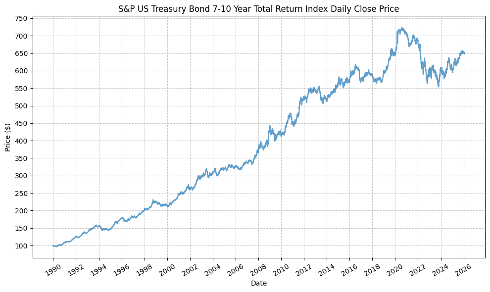
Next, we can plot the price history before calculating the cycle performance:

plot_time_series(
    df=treas_10y,
    plot_start_date=None,
    plot_end_date=None,
    plot_columns=["Close"],
    title="S&P US Treasury Bond 7-10 Year Total Return Index Daily Close Price",
    x_label="Date",
    x_format="Year",
    x_tick_spacing=2,
    x_tick_rotation=30,
    y_label="Price ($)",
    y_format="Decimal",
    y_format_decimal_places=0,
    y_tick_spacing=50,
    y_tick_rotation=0,
    grid=True,
    legend=False,
    export_plot=False,
    plot_file_name=None,
)

png

Next, we will calculate the performance for SPY based on the pre-defined Fed cycles:

treas_10y_cycles = calc_fed_cycle_asset_performance(
    start_date=cycle_ranges["start_date"],
    end_date=cycle_ranges["end_date"],
    label=cycle_ranges["cycle_label"],
    fed_funds_change=cycle_ranges["fed_funds_change"],
    monthly_returns=treas_10y_monthly,
)

display(treas_10y_cycles)

	Cycle	Start	End	Months	CumulativeReturn	CumulativeReturnPct	AverageMonthlyReturn	AverageMonthlyReturnPct	AnnualizedReturn	AnnualizedReturnPct	Volatility	FedFundsChange	FedFundsChange_bps	FFR_AnnualizedChange	FFR_AnnualizedChange_bps	Label
0	Cycle 1	1989-12-31	1990-06-30	6	0.01	1.36	0.00	0.24	0.03	2.74	0.07	0.00	0.00	0.00	0.00	Cycle 1, 1989-12-31 to 1990-06-30
1	Cycle 2	1990-06-30	1993-03-31	34	0.46	45.68	0.01	1.12	0.14	14.20	0.05	-0.05	-525.00	-0.02	-185.29	Cycle 2, 1990-06-30 to 1993-03-31
2	Cycle 3	1993-03-31	1994-01-31	11	0.09	8.88	0.01	0.78	0.10	9.72	0.04	0.00	0.00	0.00	0.00	Cycle 3, 1993-03-31 to 1994-01-31
3	Cycle 4	1994-01-31	1995-06-30	18	0.08	7.80	0.00	0.44	0.05	5.13	0.07	0.03	300.00	0.02	200.00	Cycle 4, 1994-01-31 to 1995-06-30
4	Cycle 5	1995-06-30	1996-07-31	14	0.05	4.78	0.00	0.34	0.04	4.09	0.05	-0.01	-75.00	-0.01	-64.29	Cycle 5, 1995-06-30 to 1996-07-31
5	Cycle 6	1996-07-31	1997-02-28	8	0.05	5.30	0.01	0.66	0.08	8.06	0.05	0.00	0.00	0.00	0.00	Cycle 6, 1996-07-31 to 1997-02-28
6	Cycle 7	1997-02-28	1997-09-30	8	0.06	6.45	0.01	0.80	0.10	9.83	0.06	0.00	25.00	0.00	37.50	Cycle 7, 1997-02-28 to 1997-09-30
7	Cycle 8	1997-09-30	1998-08-31	12	0.14	14.43	0.01	1.14	0.14	14.43	0.04	0.00	0.00	0.00	0.00	Cycle 8, 1997-09-30 to 1998-08-31
8	Cycle 9	1998-08-31	1999-05-31	10	0.03	3.05	0.00	0.33	0.04	3.67	0.08	-0.01	-75.00	-0.01	-90.00	Cycle 9, 1998-08-31 to 1999-05-31
9	Cycle 10	1999-05-31	2000-11-30	19	0.09	8.74	0.00	0.45	0.05	5.44	0.04	0.02	175.00	0.01	110.53	Cycle 10, 1999-05-31 to 2000-11-30
10	Cycle 11	2000-11-30	2000-12-31	2	0.05	4.92	0.02	2.43	0.33	33.39	0.00	0.00	0.00	0.00	0.00	Cycle 11, 2000-11-30 to 2000-12-31
11	Cycle 12	2000-12-31	2002-06-30	19	0.14	14.33	0.01	0.72	0.09	8.83	0.06	-0.05	-475.00	-0.03	-300.00	Cycle 12, 2000-12-31 to 2002-06-30
12	Cycle 13	2002-06-30	2002-10-31	5	0.10	9.94	0.02	1.93	0.26	25.55	0.07	0.00	0.00	0.00	0.00	Cycle 13, 2002-06-30 to 2002-10-31
13	Cycle 14	2002-10-31	2003-12-31	15	0.02	2.16	0.00	0.17	0.02	1.73	0.09	-0.01	-75.00	-0.01	-60.00	Cycle 14, 2002-10-31 to 2003-12-31
14	Cycle 15	2003-12-31	2004-05-31	6	-0.00	-0.09	0.00	0.01	-0.00	-0.18	0.08	0.00	0.00	0.00	0.00	Cycle 15, 2003-12-31 to 2004-05-31
15	Cycle 16	2004-05-31	2006-12-31	32	0.10	10.27	0.00	0.31	0.04	3.73	0.04	0.04	425.00	0.02	159.38	Cycle 16, 2004-05-31 to 2006-12-31
16	Cycle 17	2006-12-31	2007-08-31	9	0.03	3.30	0.00	0.37	0.04	4.42	0.05	0.00	0.00	0.00	0.00	Cycle 17, 2006-12-31 to 2007-08-31
17	Cycle 18	2007-08-31	2009-07-31	24	0.20	19.84	0.01	0.79	0.09	9.47	0.09	-0.05	-500.00	-0.03	-250.00	Cycle 18, 2007-08-31 to 2009-07-31
18	Cycle 19	2009-07-31	2015-11-30	77	0.39	38.99	0.00	0.44	0.05	5.27	0.06	0.00	0.00	0.00	0.00	Cycle 19, 2009-07-31 to 2015-11-30
19	Cycle 20	2015-11-30	2016-06-30	8	0.07	6.79	0.01	0.83	0.10	10.36	0.05	0.00	25.00	0.00	37.50	Cycle 20, 2015-11-30 to 2016-06-30
20	Cycle 21	2016-06-30	2016-11-30	6	-0.03	-3.17	-0.01	-0.51	-0.06	-6.25	0.08	0.00	0.00	0.00	0.00	Cycle 21, 2016-06-30 to 2016-11-30
21	Cycle 22	2016-11-30	2019-06-30	32	0.06	5.92	0.00	0.19	0.02	2.18	0.05	0.02	200.00	0.01	75.00	Cycle 22, 2016-11-30 to 2019-06-30
22	Cycle 23	2019-06-30	2019-07-31	2	0.01	1.31	0.01	0.65	0.08	8.09	0.03	0.00	0.00	0.00	0.00	Cycle 23, 2019-06-30 to 2019-07-31
23	Cycle 24	2019-07-31	2020-09-30	15	0.13	13.08	0.01	0.84	0.10	10.34	0.06	-0.02	-225.00	-0.02	-180.00	Cycle 24, 2019-07-31 to 2020-09-30
24	Cycle 25	2020-09-30	2022-02-28	18	-0.07	-6.52	-0.00	-0.37	-0.04	-4.40	0.04	0.00	0.00	0.00	0.00	Cycle 25, 2020-09-30 to 2022-02-28
25	Cycle 26	2022-02-28	2024-01-31	24	-0.10	-9.88	-0.00	-0.39	-0.05	-5.07	0.10	0.05	525.00	0.03	262.50	Cycle 26, 2022-02-28 to 2024-01-31
26	Cycle 27	2024-01-31	2024-08-31	8	0.03	2.75	0.00	0.36	0.04	4.15	0.07	0.00	0.00	0.00	0.00	Cycle 27, 2024-01-31 to 2024-08-31
27	Cycle 28	2024-08-31	2025-06-30	11	0.03	3.29	0.00	0.31	0.04	3.60	0.06	-0.01	-100.00	-0.01	-109.09	Cycle 28, 2024-08-31 to 2025-06-30
28	Cycle 29	2025-06-30	2025-08-31	3	0.03	2.67	0.01	0.89	0.11	11.11	0.04	0.00	0.00	0.00	0.00	Cycle 29, 2025-06-30 to 2025-08-31
29	Cycle 30	2025-08-31	2026-01-31	6	0.03	3.08	0.01	0.51	0.06	6.26	0.03	-0.01	-75.00	-0.01	-150.00	Cycle 30, 2025-08-31 to 2026-01-31

This gives us the following data points:

Cycle start date
Cycle end date
Number of months in the cycle
Cumulative return during the cycle (decimal and percent)
Average monthly return during the cycle (decimal and percent)
Annualized return during the cycle (decimal and percent)
Return volatility during the cycle
Cumulative change in FFR during the cycle (decimal and basis points)
Annualized change in FFR during the cycle (decimal and basis points)

From the above DataFrame, we can then plot the cumulative and annualized returns for each cycle in a bar chart. First, the cumulative returns along with the cumulative change in FFR:

plot_bar_returns_ffr_change(
    cycle_df=treas_10y_cycles,
    asset_label="TREAS_10Y",
    annualized_or_cumulative="Cumulative",
)

png

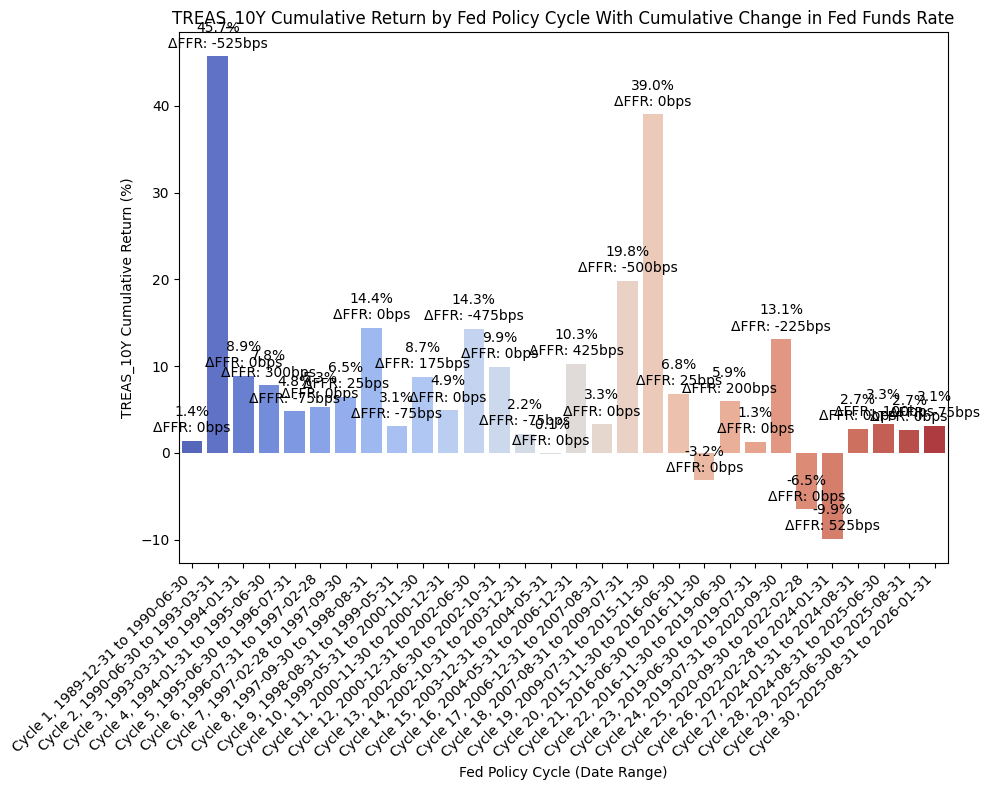
And then the annualized returns along with the annualized change in FFR:

plot_bar_returns_ffr_change(
    cycle_df=treas_10y_cycles,
    asset_label="TREAS_10Y",
    annualized_or_cumulative="Annualized",
)

png

For this dataset, we have cycles 11/12/13/14 exhibiting strong returns, which is consistent with the economic intuition that bonds should perform well during periods of economic weakness and rate cuts. We also see this outcome with cycle 18. It becomes a little more interesting during cycles 25 and 26, where the correlations of stocks and bond returns seemed to align, so we see negative bond returns there. Finally, cycles 28/29/30 also exhibit positive bond returns, which is consistent with our thesis that bonds should perform well during periods of economic weakness and rate cuts.

Finally, we can run an OLS regression to check fit:

df = treas_10y_cycles

#=== Don't modify below this line ===

# Run OLS regression with statsmodels
X = df["FFR_AnnualizedChange_bps"]
y = df["AnnualizedReturnPct"]
X = sm.add_constant(X)
model = sm.OLS(y, X).fit()
print(model.summary())
print(f"Intercept: {model.params[0]}, Slope: {model.params[1]}")  # Intercept and slope

# Calc X and Y values for regression line
X_vals = np.linspace(X.min(), X.max(), 100)
Y_vals = model.params[0] + model.params[1] * X_vals

                             OLS Regression Results                            
===============================================================================
Dep. Variable:     AnnualizedReturnPct   R-squared:                       0.050
Model:                             OLS   Adj. R-squared:                  0.016
Method:                  Least Squares   F-statistic:                     1.462
Date:                 Mon, 23 Mar 2026   Prob (F-statistic):              0.237
Time:                         22:08:23   Log-Likelihood:                -103.64
No. Observations:                   30   AIC:                             211.3
Df Residuals:                       28   BIC:                             214.1
Df Model:                            1                                         
Covariance Type:             nonrobust                                         
============================================================================================
                               coef    std err          t      P>|t|      [0.025      0.975]
--------------------------------------------------------------------------------------------
const                        6.7457      1.462      4.613      0.000       3.751       9.741
FFR_AnnualizedChange_bps    -0.0149      0.012     -1.209      0.237      -0.040       0.010
==============================================================================
Omnibus:                       19.978   Durbin-Watson:                   2.116
Prob(Omnibus):                  0.000   Jarque-Bera (JB):               29.185
Skew:                           1.582   Prob(JB):                     4.60e-07
Kurtosis:                       6.651   Cond. No.                         120.
==============================================================================

Notes:
[1] Standard Errors assume that the covariance matrix of the errors is correctly specified.
Intercept: 6.745718627069434, Slope: -0.01486255000436152

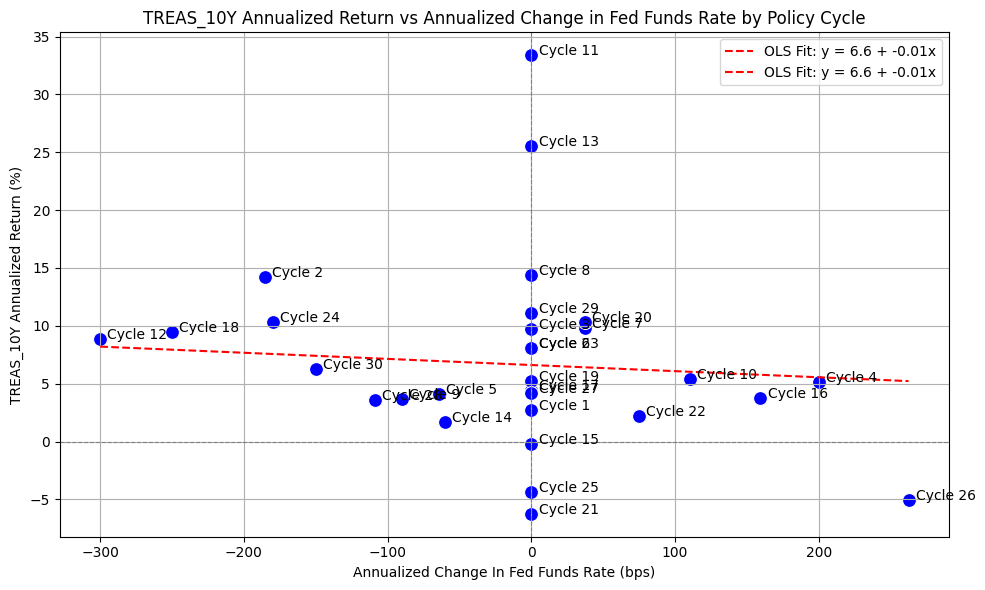
And then plot the regression line along with the values:

plot_scatter_regression_ffr_vs_returns(
    cycle_df=treas_10y_cycles,
    asset_label="TREAS_10Y",
    x_vals=X_vals,
    y_vals=Y_vals,
    intercept=model.params[0],
    slope=model.params[1],
)

png

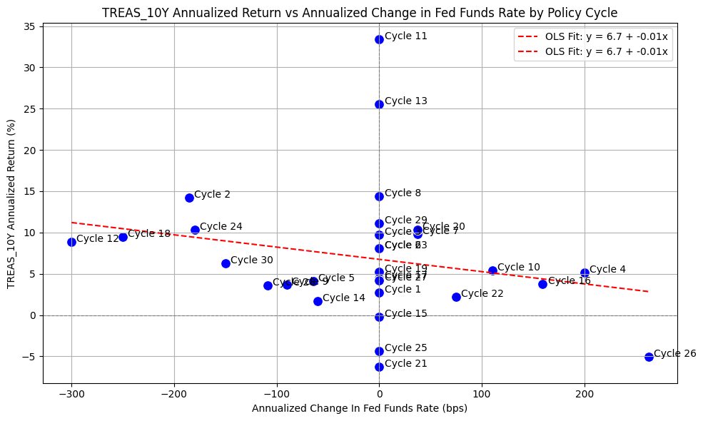
The above plot is intriguing because of how well the OLS regression appears to fit the data. It certainly appears that during rate-cutting cycles, bonds are an asset that performs well.

High Yield Bonds #

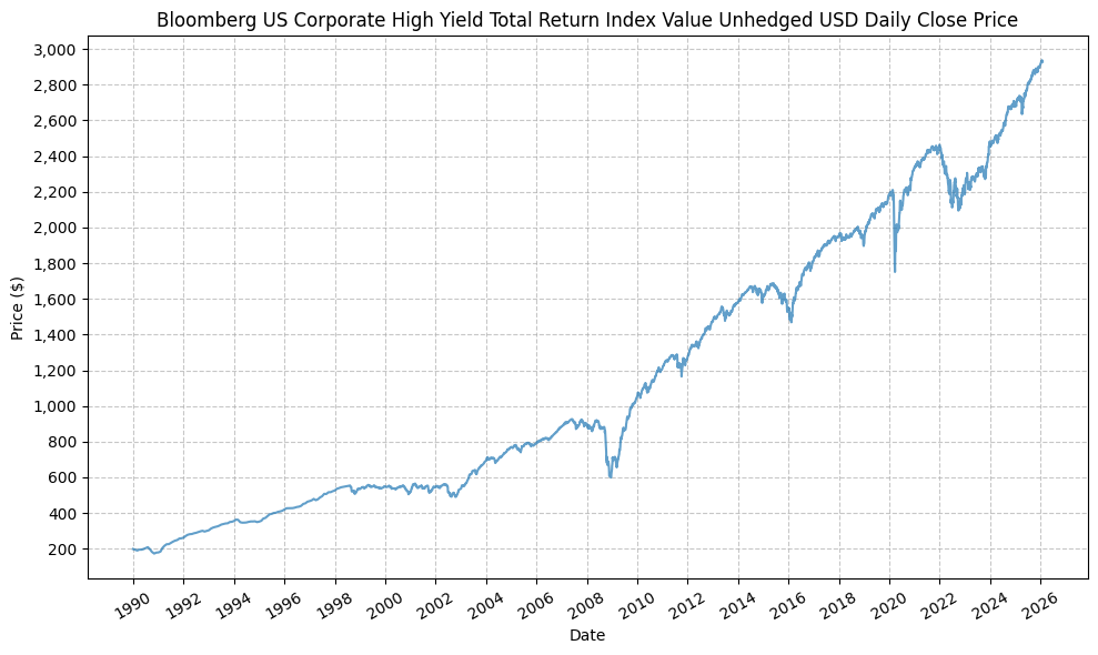
Next, we’ll run a similar process for high yield bonds using LF98TRUU_Bloomberg US Corporate High Yield Total Return Index Value Unhedged USD.

First, we pull data with the following:

bb_clean_data(
    base_directory=DATA_DIR,
    fund_ticker_name="LF98TRUU_Bloomberg US Corporate High Yield Total Return Index Value Unhedged USD",
    source="Bloomberg",
    asset_class="Indices",
    excel_export=True,
    pickle_export=True,
    output_confirmation=False,
)

hy_bonds = load_data(
    base_directory=DATA_DIR,
    ticker="LF98TRUU_Bloomberg US Corporate High Yield Total Return Index Value Unhedged USD_Clean",
    source="Bloomberg", 
    asset_class="Indices",
    timeframe="Daily",
    file_format="pickle",
)

# Filter HY_BONDS to date range
hy_bonds = hy_bonds[(hy_bonds.index >= pd.to_datetime(start_date)) & (hy_bonds.index <= pd.to_datetime(end_date))]

# Drop everything except the "close" column
hy_bonds = hy_bonds[["Close"]]

# Resample to monthly frequency
hy_bonds_monthly = hy_bonds.resample("M").last()
hy_bonds_monthly["Monthly_Return"] = hy_bonds_monthly["Close"].pct_change()
hy_bonds_monthly = hy_bonds_monthly.dropna()

display(hy_bonds_monthly)

	Close	Monthly_Return
Date
1990-01-31	194.21	-0.02
1990-02-28	190.20	-0.02
1990-03-31	195.19	0.03
1990-04-30	194.86	-0.00
1990-05-31	198.62	0.02
...	...	...
2025-09-30	2876.85	0.01
2025-10-31	2881.38	0.00
2025-11-30	2898.07	0.01
2025-12-31	2914.49	0.01
2026-01-31	2929.32	0.01

433 rows × 2 columns

Next, we can plot the price history before calculating the cycle performance:

plot_time_series(
    df=hy_bonds,
    plot_start_date=None,
    plot_end_date=None,
    plot_columns=["Close"],
    title="Bloomberg US Corporate High Yield Total Return Index Value Unhedged USD Daily Close Price",
    x_label="Date",
    x_format="Year",
    x_tick_spacing=2,
    x_tick_rotation=30,
    y_label="Price ($)",
    y_format="Decimal",
    y_format_decimal_places=0,
    y_tick_spacing=200,
    y_tick_rotation=0,
    grid=True,
    legend=False,
    export_plot=False,
    plot_file_name=None,
)

png

Next, we will calculate the performance of high yield bonds based on the pre-defined Fed cycles:

hy_bonds_cycles = calc_fed_cycle_asset_performance(
    start_date=cycle_ranges["start_date"],
    end_date=cycle_ranges["end_date"],
    label=cycle_ranges["cycle_label"],
    fed_funds_change=cycle_ranges["fed_funds_change"],
    monthly_returns=hy_bonds_monthly,
)

display(hy_bonds_cycles)

	Cycle	Start	End	Months	CumulativeReturn	CumulativeReturnPct	AverageMonthlyReturn	AverageMonthlyReturnPct	AnnualizedReturn	AnnualizedReturnPct	Volatility	FedFundsChange	FedFundsChange_bps	FFR_AnnualizedChange	FFR_AnnualizedChange_bps	Label
0	Cycle 1	1989-12-31	1990-06-30	6	0.02	2.49	0.00	0.43	0.05	5.05	0.08	0.00	0.00	0.00	0.00	Cycle 1, 1989-12-31 to 1990-06-30
1	Cycle 2	1990-06-30	1993-03-31	34	0.62	62.15	0.01	1.48	0.19	18.60	0.11	-0.05	-525.00	-0.02	-185.29	Cycle 2, 1990-06-30 to 1993-03-31
2	Cycle 3	1993-03-31	1994-01-31	11	0.14	14.26	0.01	1.22	0.16	15.66	0.02	0.00	0.00	0.00	0.00	Cycle 3, 1993-03-31 to 1994-01-31
3	Cycle 4	1994-01-31	1995-06-30	18	0.11	11.25	0.01	0.61	0.07	7.37	0.06	0.03	300.00	0.02	200.00	Cycle 4, 1994-01-31 to 1995-06-30
4	Cycle 5	1995-06-30	1996-07-31	14	0.11	10.89	0.01	0.74	0.09	9.27	0.02	-0.01	-75.00	-0.01	-64.29	Cycle 5, 1995-06-30 to 1996-07-31
5	Cycle 6	1996-07-31	1997-02-28	8	0.10	10.48	0.01	1.26	0.16	16.12	0.02	0.00	0.00	0.00	0.00	Cycle 6, 1996-07-31 to 1997-02-28
6	Cycle 7	1997-02-28	1997-09-30	8	0.10	9.56	0.01	1.16	0.15	14.67	0.05	0.00	25.00	0.00	37.50	Cycle 7, 1997-02-28 to 1997-09-30
7	Cycle 8	1997-09-30	1998-08-31	12	0.03	3.22	0.00	0.28	0.03	3.22	0.07	0.00	0.00	0.00	0.00	Cycle 8, 1997-09-30 to 1998-08-31
8	Cycle 9	1998-08-31	1999-05-31	10	-0.01	-0.73	-0.00	-0.04	-0.01	-0.87	0.09	-0.01	-75.00	-0.01	-90.00	Cycle 9, 1998-08-31 to 1999-05-31
9	Cycle 10	1999-05-31	2000-11-30	19	-0.09	-8.92	-0.00	-0.48	-0.06	-5.73	0.05	0.02	175.00	0.01	110.53	Cycle 10, 1999-05-31 to 2000-11-30
10	Cycle 11	2000-11-30	2000-12-31	2	-0.02	-2.11	-0.01	-1.01	-0.12	-11.98	0.14	0.00	0.00	0.00	0.00	Cycle 11, 2000-11-30 to 2000-12-31
11	Cycle 12	2000-12-31	2002-06-30	19	0.02	2.12	0.00	0.17	0.01	1.33	0.12	-0.05	-475.00	-0.03	-300.00	Cycle 12, 2000-12-31 to 2002-06-30
12	Cycle 13	2002-06-30	2002-10-31	5	-0.11	-10.87	-0.02	-2.22	-0.24	-24.14	0.13	0.00	0.00	0.00	0.00	Cycle 13, 2002-06-30 to 2002-10-31
13	Cycle 14	2002-10-31	2003-12-31	15	0.38	37.66	0.02	2.17	0.29	29.14	0.07	-0.01	-75.00	-0.01	-60.00	Cycle 14, 2002-10-31 to 2003-12-31
14	Cycle 15	2003-12-31	2004-05-31	6	0.02	2.19	0.00	0.37	0.04	4.42	0.05	0.00	0.00	0.00	0.00	Cycle 15, 2003-12-31 to 2004-05-31
15	Cycle 16	2004-05-31	2006-12-31	32	0.26	25.62	0.01	0.72	0.09	8.93	0.04	0.04	425.00	0.02	159.38	Cycle 16, 2004-05-31 to 2006-12-31
16	Cycle 17	2006-12-31	2007-08-31	9	0.02	1.68	0.00	0.20	0.02	2.25	0.06	0.00	0.00	0.00	0.00	Cycle 17, 2006-12-31 to 2007-08-31
17	Cycle 18	2007-08-31	2009-07-31	24	0.05	4.91	0.00	0.37	0.02	2.42	0.20	-0.05	-500.00	-0.03	-250.00	Cycle 18, 2007-08-31 to 2009-07-31
18	Cycle 19	2009-07-31	2015-11-30	77	0.83	83.15	0.01	0.81	0.10	9.89	0.07	0.00	0.00	0.00	0.00	Cycle 19, 2009-07-31 to 2015-11-30
19	Cycle 20	2015-11-30	2016-06-30	8	0.04	3.95	0.01	0.52	0.06	5.98	0.09	0.00	25.00	0.00	37.50	Cycle 20, 2015-11-30 to 2016-06-30
20	Cycle 21	2016-06-30	2016-11-30	6	0.06	6.43	0.01	1.05	0.13	13.27	0.04	0.00	0.00	0.00	0.00	Cycle 21, 2016-06-30 to 2016-11-30
21	Cycle 22	2016-11-30	2019-06-30	32	0.17	17.31	0.01	0.51	0.06	6.17	0.04	0.02	200.00	0.01	75.00	Cycle 22, 2016-11-30 to 2019-06-30
22	Cycle 23	2019-06-30	2019-07-31	2	0.03	2.86	0.01	1.42	0.18	18.41	0.04	0.00	0.00	0.00	0.00	Cycle 23, 2019-06-30 to 2019-07-31
23	Cycle 24	2019-07-31	2020-09-30	15	0.05	4.63	0.00	0.37	0.04	3.69	0.13	-0.02	-225.00	-0.02	-180.00	Cycle 24, 2019-07-31 to 2020-09-30
24	Cycle 25	2020-09-30	2022-02-28	18	0.07	6.77	0.00	0.37	0.04	4.47	0.05	0.00	0.00	0.00	0.00	Cycle 25, 2020-09-30 to 2022-02-28
25	Cycle 26	2022-02-28	2024-01-31	24	0.04	3.58	0.00	0.19	0.02	1.77	0.10	0.05	525.00	0.03	262.50	Cycle 26, 2022-02-28 to 2024-01-31
26	Cycle 27	2024-01-31	2024-08-31	8	0.06	6.28	0.01	0.77	0.10	9.57	0.03	0.00	0.00	0.00	0.00	Cycle 27, 2024-01-31 to 2024-08-31
27	Cycle 28	2024-08-31	2025-06-30	11	0.08	8.18	0.01	0.72	0.09	8.96	0.04	-0.01	-100.00	-0.01	-109.09	Cycle 28, 2024-08-31 to 2025-06-30
28	Cycle 29	2025-06-30	2025-08-31	3	0.04	3.58	0.01	1.18	0.15	15.09	0.02	0.00	0.00	0.00	0.00	Cycle 29, 2025-06-30 to 2025-08-31
29	Cycle 30	2025-08-31	2026-01-31	6	0.04	3.94	0.01	0.65	0.08	8.03	0.01	-0.01	-75.00	-0.01	-150.00	Cycle 30, 2025-08-31 to 2026-01-31

This gives us the following data points:

Cycle start date
Cycle end date
Number of months in the cycle
Cumulative return during the cycle (decimal and percent)
Average monthly return during the cycle (decimal and percent)
Annualized return during the cycle (decimal and percent)
Return volatility during the cycle
Cumulative change in FFR during the cycle (decimal and basis points)
Annualized change in FFR during the cycle (decimal and basis points)

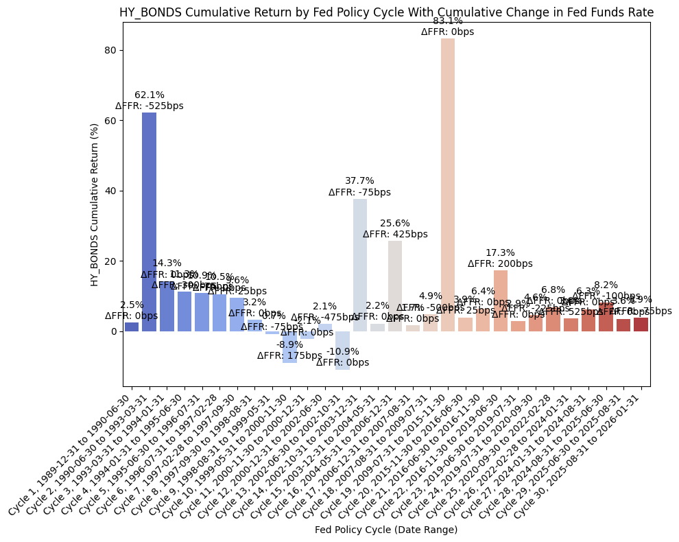
From the above DataFrame, we can then plot the cumulative and annualized returns for each cycle in a bar chart. First, the cumulative returns along with the cumulative change in FFR:

plot_bar_returns_ffr_change(
    cycle_df=hy_bonds_cycles,
    asset_label="HY_BONDS",
    annualized_or_cumulative="Cumulative",
)

png

And then the annualized returns along with the annualized change in FFR:

plot_bar_returns_ffr_change(
    cycle_df=hy_bonds_cycles,
    asset_label="HY_BONDS",
    annualized_or_cumulative="Annualized",
)

png

Finally, we can run an OLS regression to check fit:

df = hy_bonds_cycles

#=== Don't modify below this line ===

# Run OLS regression with statsmodels
X = df["FFR_AnnualizedChange_bps"]
y = df["AnnualizedReturnPct"]
X = sm.add_constant(X)
model = sm.OLS(y, X).fit()
print(model.summary())
print(f"Intercept: {model.params[0]}, Slope: {model.params[1]}")  # Intercept and slope

# Calc X and Y values for regression line
X_vals = np.linspace(X.min(), X.max(), 100)
Y_vals = model.params[0] + model.params[1] * X_vals

                             OLS Regression Results                            
===============================================================================
Dep. Variable:     AnnualizedReturnPct   R-squared:                       0.004
Model:                             OLS   Adj. R-squared:                 -0.031
Method:                  Least Squares   F-statistic:                    0.1171
Date:                 Mon, 23 Mar 2026   Prob (F-statistic):              0.735
Time:                         22:08:25   Log-Likelihood:                -110.57
No. Observations:                   30   AIC:                             225.1
Df Residuals:                       28   BIC:                             227.9
Df Model:                            1                                         
Covariance Type:             nonrobust                                         
============================================================================================
                               coef    std err          t      P>|t|      [0.025      0.975]
--------------------------------------------------------------------------------------------
const                        6.6113      1.842      3.590      0.001       2.839      10.384
FFR_AnnualizedChange_bps    -0.0053      0.015     -0.342      0.735      -0.037       0.026
==============================================================================
Omnibus:                        9.087   Durbin-Watson:                   1.936
Prob(Omnibus):                  0.011   Jarque-Bera (JB):                9.047
Skew:                          -0.790   Prob(JB):                       0.0109
Kurtosis:                       5.178   Cond. No.                         120.
==============================================================================

Notes:
[1] Standard Errors assume that the covariance matrix of the errors is correctly specified.
Intercept: 6.611340605920211, Slope: -0.005299161729553994

And then plot the regression line along with the values:

plot_scatter_regression_ffr_vs_returns(
    cycle_df=treas_10y_cycles,
    asset_label="TREAS_10Y",
    x_vals=X_vals,
    y_vals=Y_vals,
    intercept=model.params[0],
    slope=model.params[1],
)

png

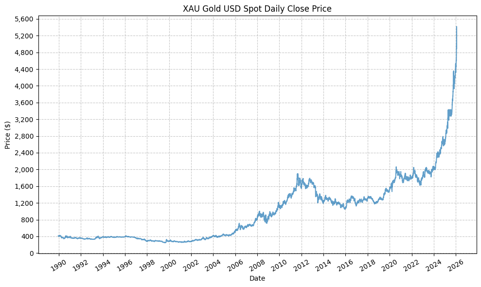
Gold #

Finally, we’ll run a similar process for gold using XAU_Gold USD Spot.

First, we pull data with the following:

bb_clean_data(
    base_directory=DATA_DIR,
    fund_ticker_name="XAU_Gold USD Spot",
    source="Bloomberg",
    asset_class="Commodities",
    excel_export=True,
    pickle_export=True,
    output_confirmation=False,
)

gold = load_data(
    base_directory=DATA_DIR,
    ticker="XAU_Gold USD Spot_Clean",
    source="Bloomberg", 
    asset_class="Commodities",
    timeframe="Daily",
    file_format="pickle",
)

# Filter GOLD to date range
gold = gold[(gold.index >= pd.to_datetime(start_date)) & (gold.index <= pd.to_datetime(end_date))]

# Drop everything except the "close" column
gold = gold[["Close"]]

# Resample to monthly frequency
gold_monthly = gold.resample("M").last()
gold_monthly["Monthly_Return"] = gold_monthly["Close"].pct_change()
gold_monthly = gold_monthly.dropna()

display(gold_monthly)

	Close	Monthly_Return
Date
1990-01-31	415.05	0.03
1990-02-28	407.70	-0.02
1990-03-31	368.50	-0.10
1990-04-30	367.75	-0.00
1990-05-31	363.05	-0.01
...	...	...
2025-09-30	3858.96	0.12
2025-10-31	4002.92	0.04
2025-11-30	4239.43	0.06
2025-12-31	4319.37	0.02
2026-01-31	4894.23	0.13

433 rows × 2 columns

Next, we can plot the price history before calculating the cycle performance:

plot_time_series(
    df=gold,
    plot_start_date=None,
    plot_end_date=None,
    plot_columns=["Close"],
    title="XAU Gold USD Spot Daily Close Price",
    x_label="Date",
    x_format="Year",
    x_tick_spacing=2,
    x_tick_rotation=30,
    y_label="Price ($)",
    y_format="Decimal",
    y_format_decimal_places=0,
    y_tick_spacing=400,
    y_tick_rotation=0,
    grid=True,
    legend=False,
    export_plot=False,
    plot_file_name=None,
)

png

Next, we will calculate the performance of gold based on the pre-defined Fed cycles:

gold_cycles = calc_fed_cycle_asset_performance(
    start_date=cycle_ranges["start_date"],
    end_date=cycle_ranges["end_date"],
    label=cycle_ranges["cycle_label"],
    fed_funds_change=cycle_ranges["fed_funds_change"],
    monthly_returns=gold_monthly,
)

display(gold_cycles)

	Cycle	Start	End	Months	CumulativeReturn	CumulativeReturnPct	AverageMonthlyReturn	AverageMonthlyReturnPct	AnnualizedReturn	AnnualizedReturnPct	Volatility	FedFundsChange	FedFundsChange_bps	FFR_AnnualizedChange	FFR_AnnualizedChange_bps	Label
0	Cycle 1	1989-12-31	1990-06-30	6	-0.12	-12.22	-0.02	-2.07	-0.23	-22.95	0.15	0.00	0.00	0.00	0.00	Cycle 1, 1989-12-31 to 1990-06-30
1	Cycle 2	1990-06-30	1993-03-31	34	-0.07	-6.62	-0.00	-0.16	-0.02	-2.39	0.10	-0.05	-525.00	-0.02	-185.29	Cycle 2, 1990-06-30 to 1993-03-31
2	Cycle 3	1993-03-31	1994-01-31	11	0.16	15.90	0.01	1.46	0.17	17.47	0.17	0.00	0.00	0.00	0.00	Cycle 3, 1993-03-31 to 1994-01-31
3	Cycle 4	1994-01-31	1995-06-30	18	-0.02	-1.56	-0.00	-0.07	-0.01	-1.04	0.07	0.03	300.00	0.02	200.00	Cycle 4, 1994-01-31 to 1995-06-30
4	Cycle 5	1995-06-30	1996-07-31	14	0.01	0.72	0.00	0.07	0.01	0.61	0.06	-0.01	-75.00	-0.01	-64.29	Cycle 5, 1995-06-30 to 1996-07-31
5	Cycle 6	1996-07-31	1997-02-28	8	-0.04	-4.47	-0.01	-0.52	-0.07	-6.63	0.12	0.00	0.00	0.00	0.00	Cycle 6, 1996-07-31 to 1997-02-28
6	Cycle 7	1997-02-28	1997-09-30	8	-0.03	-2.87	-0.00	-0.31	-0.04	-4.28	0.12	0.00	25.00	0.00	37.50	Cycle 7, 1997-02-28 to 1997-09-30
7	Cycle 8	1997-09-30	1998-08-31	12	-0.15	-14.99	-0.01	-1.28	-0.15	-14.99	0.12	0.00	0.00	0.00	0.00	Cycle 8, 1997-09-30 to 1998-08-31
8	Cycle 9	1998-08-31	1999-05-31	10	-0.06	-5.62	-0.01	-0.52	-0.07	-6.71	0.13	-0.01	-75.00	-0.01	-90.00	Cycle 9, 1998-08-31 to 1999-05-31
9	Cycle 10	1999-05-31	2000-11-30	19	-0.06	-5.62	-0.00	-0.19	-0.04	-3.59	0.17	0.02	175.00	0.01	110.53	Cycle 10, 1999-05-31 to 2000-11-30
10	Cycle 11	2000-11-30	2000-12-31	2	0.03	2.68	0.01	1.33	0.17	17.18	0.03	0.00	0.00	0.00	0.00	Cycle 11, 2000-11-30 to 2000-12-31
11	Cycle 12	2000-12-31	2002-06-30	19	0.16	16.27	0.01	0.84	0.10	9.99	0.11	-0.05	-475.00	-0.03	-300.00	Cycle 12, 2000-12-31 to 2002-06-30
12	Cycle 13	2002-06-30	2002-10-31	5	-0.03	-2.69	-0.00	-0.50	-0.06	-6.35	0.12	0.00	0.00	0.00	0.00	Cycle 13, 2002-06-30 to 2002-10-31
13	Cycle 14	2002-10-31	2003-12-31	15	0.28	28.40	0.02	1.77	0.22	22.14	0.15	-0.01	-75.00	-0.01	-60.00	Cycle 14, 2002-10-31 to 2003-12-31
14	Cycle 15	2003-12-31	2004-05-31	6	-0.01	-0.65	0.00	0.04	-0.01	-1.30	0.21	0.00	0.00	0.00	0.00	Cycle 15, 2003-12-31 to 2004-05-31
15	Cycle 16	2004-05-31	2006-12-31	32	0.65	64.63	0.02	1.65	0.21	20.56	0.15	0.04	425.00	0.02	159.38	Cycle 16, 2004-05-31 to 2006-12-31
16	Cycle 17	2006-12-31	2007-08-31	9	0.04	3.90	0.00	0.45	0.05	5.24	0.07	0.00	0.00	0.00	0.00	Cycle 17, 2006-12-31 to 2007-08-31
17	Cycle 18	2007-08-31	2009-07-31	24	0.44	43.61	0.02	1.77	0.20	19.84	0.25	-0.05	-500.00	-0.03	-250.00	Cycle 18, 2007-08-31 to 2009-07-31
18	Cycle 19	2009-07-31	2015-11-30	77	0.15	14.92	0.00	0.32	0.02	2.19	0.18	0.00	0.00	0.00	0.00	Cycle 19, 2009-07-31 to 2015-11-30
19	Cycle 20	2015-11-30	2016-06-30	8	0.16	15.74	0.02	2.03	0.25	24.52	0.23	0.00	25.00	0.00	37.50	Cycle 20, 2015-11-30 to 2016-06-30
20	Cycle 21	2016-06-30	2016-11-30	6	-0.03	-3.47	-0.00	-0.45	-0.07	-6.81	0.20	0.00	0.00	0.00	0.00	Cycle 21, 2016-06-30 to 2016-11-30
21	Cycle 22	2016-11-30	2019-06-30	32	0.10	10.36	0.00	0.36	0.04	3.77	0.11	0.02	200.00	0.01	75.00	Cycle 22, 2016-11-30 to 2019-06-30
22	Cycle 23	2019-06-30	2019-07-31	2	0.08	8.29	0.04	4.13	0.61	61.24	0.19	0.00	0.00	0.00	0.00	Cycle 23, 2019-06-30 to 2019-07-31
23	Cycle 24	2019-07-31	2020-09-30	15	0.34	33.79	0.02	2.04	0.26	26.22	0.15	-0.02	-225.00	-0.02	-180.00	Cycle 24, 2019-07-31 to 2020-09-30
24	Cycle 25	2020-09-30	2022-02-28	18	-0.03	-2.99	-0.00	-0.08	-0.02	-2.00	0.15	0.00	0.00	0.00	0.00	Cycle 25, 2020-09-30 to 2022-02-28
25	Cycle 26	2022-02-28	2024-01-31	24	0.13	13.49	0.01	0.61	0.07	6.53	0.14	0.05	525.00	0.03	262.50	Cycle 26, 2022-02-28 to 2024-01-31
26	Cycle 27	2024-01-31	2024-08-31	8	0.21	21.35	0.02	2.49	0.34	33.68	0.11	0.00	0.00	0.00	0.00	Cycle 27, 2024-01-31 to 2024-08-31
27	Cycle 28	2024-08-31	2025-06-30	11	0.35	34.95	0.03	2.82	0.39	38.68	0.13	-0.01	-100.00	-0.01	-109.09	Cycle 28, 2024-08-31 to 2025-06-30
28	Cycle 29	2025-06-30	2025-08-31	3	0.05	4.82	0.02	1.61	0.21	20.74	0.10	0.00	0.00	0.00	0.00	Cycle 29, 2025-06-30 to 2025-08-31
29	Cycle 30	2025-08-31	2026-01-31	6	0.49	48.76	0.07	6.93	1.21	121.31	0.16	-0.01	-75.00	-0.01	-150.00	Cycle 30, 2025-08-31 to 2026-01-31

This gives us the following data points:

Cycle start date
Cycle end date
Number of months in the cycle
Cumulative return during the cycle (decimal and percent)
Average monthly return during the cycle (decimal and percent)
Annualized return during the cycle (decimal and percent)
Return volatility during the cycle
Cumulative change in FFR during the cycle (decimal and basis points)
Annualized change in FFR during the cycle (decimal and basis points)

From the above DataFrame, we can then plot the cumulative and annualized returns for each cycle in a bar chart. First, the cumulative returns along with the cumulative change in FFR:

plot_bar_returns_ffr_change(
    cycle_df=gold_cycles,
    asset_label="GOLD",
    annualized_or_cumulative="Cumulative",
)

png

And then the annualized returns along with the annualized change in FFR:

plot_bar_returns_ffr_change(
    cycle_df=gold_cycles,
    asset_label="GOLD",
    annualized_or_cumulative="Annualized",
)

png

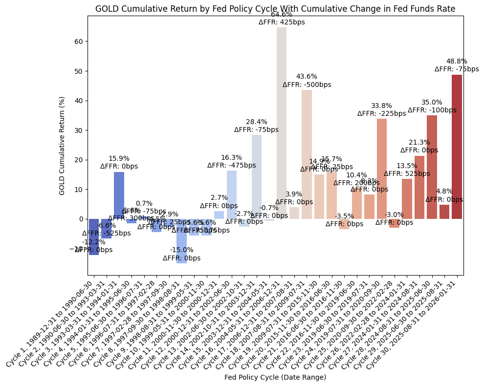
We see strong returns for gold across several different Fed cycles, so it is difficult to draw any kind of initial conclusion based on the bar charts.

Finally, we can run an OLS regression to check fit:

df = gold_cycles

#=== Don't modify below this line ===

# Run OLS regression with statsmodels
X = df["FFR_AnnualizedChange_bps"]
y = df["AnnualizedReturnPct"]
X = sm.add_constant(X)
model = sm.OLS(y, X).fit()
print(model.summary())
print(f"Intercept: {model.params[0]}, Slope: {model.params[1]}")  # Intercept and slope

# Calc X and Y values for regression line
X_vals = np.linspace(X.min(), X.max(), 100)
Y_vals = model.params[0] + model.params[1] * X_vals

                             OLS Regression Results                            
===============================================================================
Dep. Variable:     AnnualizedReturnPct   R-squared:                       0.064
Model:                             OLS   Adj. R-squared:                  0.030
Method:                  Least Squares   F-statistic:                     1.900
Date:                 Mon, 23 Mar 2026   Prob (F-statistic):              0.179
Time:                         22:08:28   Log-Likelihood:                -140.03
No. Observations:                   30   AIC:                             284.1
Df Residuals:                       28   BIC:                             286.9
Df Model:                            1                                         
Covariance Type:             nonrobust                                         
============================================================================================
                               coef    std err          t      P>|t|      [0.025      0.975]
--------------------------------------------------------------------------------------------
const                       11.4670      4.917      2.332      0.027       1.396      21.539
FFR_AnnualizedChange_bps    -0.0570      0.041     -1.378      0.179      -0.142       0.028
==============================================================================
Omnibus:                       28.991   Durbin-Watson:                   1.081
Prob(Omnibus):                  0.000   Jarque-Bera (JB):               62.894
Skew:                           2.093   Prob(JB):                     2.20e-14
Kurtosis:                       8.727   Cond. No.                         120.
==============================================================================

Notes:
[1] Standard Errors assume that the covariance matrix of the errors is correctly specified.
Intercept: 11.467013480569243, Slope: -0.056974234027166226

And then plot the regression line along with the values:

plot_scatter_regression_ffr_vs_returns(
    cycle_df=gold_cycles,
    asset_label="GOLD",
    x_vals=X_vals,
    y_vals=Y_vals,
    intercept=model.params[0],
    slope=model.params[1],
)

png

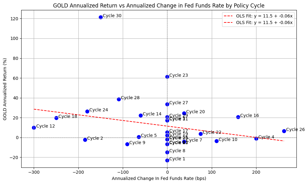
It’s difficult to draw any strong conclusions with the above plot. Gold has traditionally been considered a hedge for inflation, and while one of the Fed’s mandates is to manage inflation, there may not be a conclusion to draw in relationship to the historical returns that gold has exhibited.

Asset Allocation #

With the above analysis (somewhat) complete, let’s look at the optimal allocation for a portfolio based on the data and the hypythetical historical results.

We have to be careful with our criteria for when to hold stocks, bonds, or gold, as hindsight bias is certainly possible. So, without overanalyzing the results, let’s assume that we hold stocks as the default position during tightening cycles, and then hold bonds during easing cycles when the Fed starts cutting rates, and then resume holding stocks when the Fed stops cutting rates. If there is not any change in FFR, then we still hold stocks.

We can then combine the return series based on the above with the following:

# Shift the "cycle_filled" column down by one row to create a new column called "cycle_invested" that represents the cycle label that an investor would be invested in for each month (i.e. the cycle label from the previous month)

fedfunds_grouped_cycles['cycle_invested'] = fedfunds_grouped_cycles['cycle_filled'].shift(1)

display(fedfunds_grouped_cycles)

	start_date	fed_funds_start	end_date	fed_funds_end	fed_funds_change	cycle	cycle_filled	group	cycle_invested
0	1989-12-31	0.08	1990-01-31	0.08	0.00	Neutral	Modified Tightening	1	None
1	1990-01-31	0.08	1990-02-28	0.08	0.00	Neutral	Modified Tightening	1	Modified Tightening
2	1990-02-28	0.08	1990-03-31	0.08	0.00	Neutral	Modified Tightening	1	Modified Tightening
3	1990-03-31	0.08	1990-04-30	0.08	0.00	Neutral	Modified Tightening	1	Modified Tightening
4	1990-04-30	0.08	1990-05-31	0.08	0.00	Neutral	Modified Tightening	1	Modified Tightening
...	...	...	...	...	...	...	...	...	...
429	2025-09-30	0.04	2025-10-31	0.04	-0.00	Easing	Easing	30	Easing
430	2025-10-31	0.04	2025-11-30	0.04	0.00	Neutral	Easing	30	Easing
431	2025-11-30	0.04	2025-12-31	0.04	-0.00	Easing	Easing	30	Easing
432	2025-12-31	0.04	2026-01-31	0.04	0.00	Neutral	Easing	30	Easing
433	2026-01-31	0.04	NaT	NaN	NaN	Neutral	Easing	30	Easing

434 rows × 9 columns

# Reset index to merge on date
stocks_merged = pd.merge_asof(
    spxt_monthly.reset_index(),
    fedfunds_grouped_cycles[['start_date', 'end_date', 'cycle_invested', 'group']],
    left_on='Date',
    right_on='start_date',
    direction='backward'
)

# Drop rows where the date falls outside the cycle's end_date
stocks_merged = stocks_merged[stocks_merged['Date'] <= stocks_merged['end_date']]

display(stocks_merged)

	Date	Close	Monthly_Return	start_date	end_date	cycle_invested	group
0	1990-01-31	353.94	-0.07	1990-01-31	1990-02-28	Modified Tightening	1
1	1990-02-28	358.50	0.01	1990-02-28	1990-03-31	Modified Tightening	1
2	1990-03-31	368	0.03	1990-03-31	1990-04-30	Modified Tightening	1
3	1990-04-30	358.81	-0.02	1990-04-30	1990-05-31	Modified Tightening	1
4	1990-05-31	393.80	0.10	1990-05-31	1990-06-30	Modified Tightening	1
...	...	...	...	...	...	...	...
427	2025-08-31	14304.68	0.02	2025-08-31	2025-09-30	Modified Tightening	30
428	2025-09-30	14826.80	0.04	2025-09-30	2025-10-31	Easing	30
429	2025-10-31	15173.95	0.02	2025-10-31	2025-11-30	Easing	30
430	2025-11-30	15211.14	0.00	2025-11-30	2025-12-31	Easing	30
431	2025-12-31	15220.45	0.00	2025-12-31	2026-01-31	Easing	30

432 rows × 7 columns

# Reset index to merge on date
bonds_merged = pd.merge_asof(
    treas_10y_monthly.reset_index(),
    fedfunds_grouped_cycles[['start_date', 'end_date', 'cycle_invested', 'group']],
    left_on='Date',
    right_on='start_date',
    direction='backward'
)

# Drop rows where the date falls outside the cycle's end_date
bonds_merged = bonds_merged[bonds_merged['Date'] <= bonds_merged['end_date']]

display(bonds_merged)

	Date	Close	Monthly_Return	start_date	end_date	cycle_invested	group
0	1990-01-31	98.01	-0.02	1990-01-31	1990-02-28	Modified Tightening	1
1	1990-02-28	97.99	-0.00	1990-02-28	1990-03-31	Modified Tightening	1
2	1990-03-31	97.99	-0.00	1990-03-31	1990-04-30	Modified Tightening	1
3	1990-04-30	96.61	-0.01	1990-04-30	1990-05-31	Modified Tightening	1
4	1990-05-31	99.65	0.03	1990-05-31	1990-06-30	Modified Tightening	1
...	...	...	...	...	...	...	...
427	2025-08-31	641.26	0.02	2025-08-31	2025-09-30	Modified Tightening	30
428	2025-09-30	645.58	0.01	2025-09-30	2025-10-31	Easing	30
429	2025-10-31	650.00	0.01	2025-10-31	2025-11-30	Easing	30
430	2025-11-30	656.64	0.01	2025-11-30	2025-12-31	Easing	30
431	2025-12-31	652.29	-0.01	2025-12-31	2026-01-31	Easing	30

432 rows × 7 columns

# Select the appropriate return based on cycle
stocks_merged['strategy_return'] = stocks_merged.apply(
    lambda row: row['Monthly_Return'] if row['cycle_invested'] in ['Tightening', 'Modified Tightening'] else None,
    axis=1
)

bonds_merged['strategy_return'] = bonds_merged.apply(
    lambda row: row['Monthly_Return'] if row['cycle_invested'] == 'Easing' else None,
    axis=1
)

# Combine
strategy = pd.concat([stocks_merged, bonds_merged]).dropna(subset=['strategy_return'])
strategy = strategy.sort_values('Date')

display(strategy.head(20))

	Date	Close	Monthly_Return	start_date	end_date	cycle_invested	group	strategy_return
0	1990-01-31	353.94	-0.07	1990-01-31	1990-02-28	Modified Tightening	1	-0.07
1	1990-02-28	358.50	0.01	1990-02-28	1990-03-31	Modified Tightening	1	0.01
2	1990-03-31	368	0.03	1990-03-31	1990-04-30	Modified Tightening	1	0.03
3	1990-04-30	358.81	-0.02	1990-04-30	1990-05-31	Modified Tightening	1	-0.02
4	1990-05-31	393.80	0.10	1990-05-31	1990-06-30	Modified Tightening	1	0.10
5	1990-06-30	391.14	-0.01	1990-06-30	1990-07-31	Modified Tightening	2	-0.01
6	1990-07-31	102.84	0.01	1990-07-31	1990-08-31	Easing	2	0.01
7	1990-08-31	100.78	-0.02	1990-08-31	1990-09-30	Easing	2	-0.02
8	1990-09-30	101.74	0.01	1990-09-30	1990-10-31	Easing	2	0.01
9	1990-10-31	103.65	0.02	1990-10-31	1990-11-30	Easing	2	0.02
10	1990-11-30	106.43	0.03	1990-11-30	1990-12-31	Easing	2	0.03
11	1990-12-31	108.25	0.02	1990-12-31	1991-01-31	Easing	2	0.02
12	1991-01-31	109.53	0.01	1991-01-31	1991-02-28	Easing	2	0.01
13	1991-02-28	110.10	0.01	1991-02-28	1991-03-31	Easing	2	0.01
14	1991-03-31	110.43	0.00	1991-03-31	1991-04-30	Easing	2	0.00
15	1991-04-30	111.60	0.01	1991-04-30	1991-05-31	Easing	2	0.01
16	1991-05-31	112.08	0.00	1991-05-31	1991-06-30	Easing	2	0.00
17	1991-06-30	111.50	-0.01	1991-06-30	1991-07-31	Easing	2	-0.01
18	1991-07-31	113.05	0.01	1991-07-31	1991-08-31	Easing	2	0.01
19	1991-08-31	116.06	0.03	1991-08-31	1991-09-30	Easing	2	0.03

# Calculate cumulative returns and drawdown for spxt
spxt_monthly['Cumulative_Return'] = (1 + spxt_monthly['Monthly_Return']).cumprod() - 1
spxt_monthly['Cumulative_Return_Plus_One'] = 1 + spxt_monthly['Cumulative_Return']
spxt_monthly['Rolling_Max'] = spxt_monthly['Cumulative_Return_Plus_One'].cummax()
spxt_monthly['Drawdown'] = spxt_monthly['Cumulative_Return_Plus_One'] / spxt_monthly['Rolling_Max'] - 1
spxt_monthly.drop(columns=['Cumulative_Return_Plus_One', 'Rolling_Max'], inplace=True)

# Calculate cumulative returns and drawdown for treas_10y
treas_10y_monthly['Cumulative_Return'] = (1 + treas_10y_monthly['Monthly_Return']).cumprod() - 1
treas_10y_monthly['Cumulative_Return_Plus_One'] = 1 + treas_10y_monthly['Cumulative_Return']
treas_10y_monthly['Rolling_Max'] = treas_10y_monthly['Cumulative_Return_Plus_One'].cummax()
treas_10y_monthly['Drawdown'] = treas_10y_monthly['Cumulative_Return_Plus_One'] / treas_10y_monthly['Rolling_Max'] - 1
treas_10y_monthly.drop(columns=['Cumulative_Return_Plus_One', 'Rolling_Max'], inplace=True)

# Convert to DataFrame
portfolio_monthly = strategy[['Date', 'strategy_return']].copy().set_index('Date')
portfolio_monthly = portfolio_monthly.rename(columns={'strategy_return': 'Portfolio_Monthly_Return'})

# Calculate cumulative returns and drawdown for the portfolio
portfolio_monthly['Portfolio_Cumulative_Return'] = (1 + portfolio_monthly['Portfolio_Monthly_Return']).cumprod() - 1
portfolio_monthly['Portfolio_Cumulative_Return_Plus_One'] = 1 + portfolio_monthly['Portfolio_Cumulative_Return']
portfolio_monthly['Portfolio_Rolling_Max'] = portfolio_monthly['Portfolio_Cumulative_Return_Plus_One'].cummax()
portfolio_monthly['Portfolio_Drawdown'] = portfolio_monthly['Portfolio_Cumulative_Return_Plus_One'] / portfolio_monthly['Portfolio_Rolling_Max'] - 1
portfolio_monthly.drop(columns=['Portfolio_Cumulative_Return_Plus_One', 'Portfolio_Rolling_Max'], inplace=True)

# Merge "spxt_monthly" and "treas_10y_monthly" into "portfolio_monthly" to compare cumulative returns
portfolio_monthly = portfolio_monthly.join(
    spxt_monthly['Monthly_Return'].rename('SPXT_Monthly_Return'),
    how='left'
).join(
    spxt_monthly['Cumulative_Return'].rename('SPXT_Cumulative_Return'),
    how='left'
).join(
    spxt_monthly['Drawdown'].rename('SPXT_Drawdown'),
    how='left'
).join(
    treas_10y_monthly['Monthly_Return'].rename('10Y_Monthly_Return'),
    how='left'
).join(
    treas_10y_monthly['Cumulative_Return'].rename('10Y_Cumulative_Return'),
    how='left'
).join(
    treas_10y_monthly['Drawdown'].rename('10Y_Drawdown'),
    how='left'
)

display(portfolio_monthly)

	Portfolio_Monthly_Return	Portfolio_Cumulative_Return	Portfolio_Drawdown	SPXT_Monthly_Return	SPXT_Cumulative_Return	SPXT_Drawdown	10Y_Monthly_Return	10Y_Cumulative_Return	10Y_Drawdown
Date
1990-01-31	-0.07	-0.07	0.00	-0.07	-0.07	0.00	-0.02	-0.02	0.00
1990-02-28	0.01	-0.06	0.00	0.01	-0.06	0.00	-0.00	-0.02	-0.00
1990-03-31	0.03	-0.03	0.00	0.03	-0.03	0.00	-0.00	-0.02	-0.00
1990-04-30	-0.02	-0.05	-0.02	-0.02	-0.05	-0.02	-0.01	-0.03	-0.01
1990-05-31	0.10	0.04	0.00	0.10	0.04	0.00	0.03	-0.00	0.00
...	...	...	...	...	...	...	...	...	...
2025-08-31	0.02	42.29	0.00	0.02	36.70	0.00	0.02	5.41	-0.11
2025-09-30	0.01	42.58	0.00	0.04	38.08	0.00	0.01	5.46	-0.11
2025-10-31	0.01	42.88	0.00	0.02	38.99	0.00	0.01	5.50	-0.10
2025-11-30	0.01	43.32	0.00	0.00	39.09	0.00	0.01	5.57	-0.09
2025-12-31	-0.01	43.03	-0.01	0.00	39.12	0.00	-0.01	5.52	-0.10

432 rows × 9 columns

Next, we’ll look at performance for the assets and portfolio.

Performance Statistics #

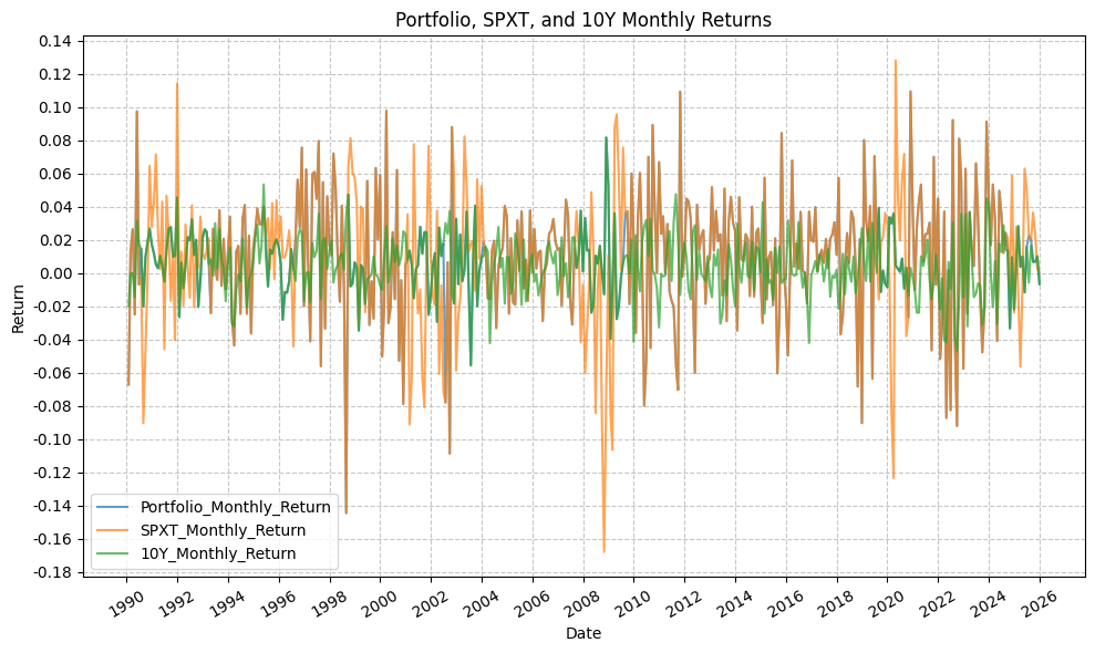
We can then plot the monthly returns:

plot_time_series(
    df=portfolio_monthly,
    plot_start_date=start_date,
    plot_end_date=end_date,
    plot_columns=["Portfolio_Monthly_Return", "SPXT_Monthly_Return", "10Y_Monthly_Return"],
    title="Portfolio, SPXT, and 10Y Monthly Returns",
    x_label="Date",
    x_format="Year",
    x_tick_spacing=2,
    x_tick_rotation=30,
    y_label="Return",
    y_format="Decimal",
    y_format_decimal_places=2,
    y_tick_spacing=0.02,
    y_tick_rotation=0,
    grid=True,
    legend=True,
    export_plot=False,
    plot_file_name=None,
)

png

And cumulative returns:

plot_time_series(
    df=portfolio_monthly,
    plot_start_date=start_date,
    plot_end_date=end_date,
    plot_columns=["Portfolio_Cumulative_Return", "SPXT_Cumulative_Return", "10Y_Cumulative_Return"],
    title="Portfolio, SPXT, and 10Y Cumulative Returns",
    x_label="Date",
    x_format="Year",
    x_tick_spacing=2,
    x_tick_rotation=30,
    y_label="Cumulative Return",
    y_format="Decimal",
    y_format_decimal_places=0,
    y_tick_spacing=3,
    y_tick_rotation=0,
    grid=True,
    legend=True,
    export_plot=False,
    plot_file_name=None,
)

png

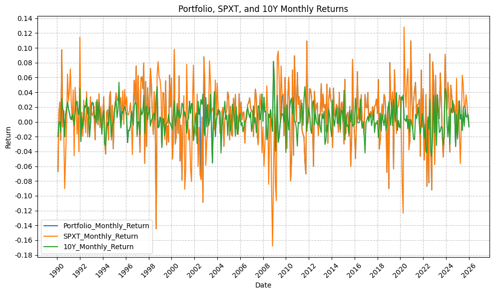
And drawdowns:

plot_time_series(
    df=portfolio_monthly,
    plot_start_date=start_date,
    plot_end_date=end_date,
    plot_columns=["Portfolio_Drawdown", "SPXT_Drawdown", "10Y_Drawdown"],
    title="Portfolio, SPXT, and 10Y Drawdowns",
    x_label="Date",
    x_format="Year",
    x_tick_spacing=2,
    x_tick_rotation=30,
    y_label="Drawdown (%)",
    y_format="Decimal",
    y_format_decimal_places=2,
    y_tick_spacing=0.05,
    y_tick_rotation=0,
    grid=True,
    legend=True,
    export_plot=False,
    plot_file_name=None,
)

png

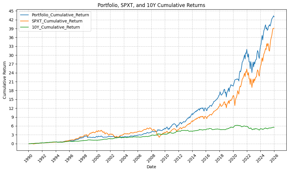
Finally, we can run the summary statistics on the strategy portfolio, SPY, and TLT with the following code:

port_sum_stats = summary_stats(
    fund_list=["Portfolio", "SPXT", "10Y"],
    df=portfolio_monthly[["Portfolio_Monthly_Return"]],
    period="Monthly",
    use_calendar_days=False,
    excel_export=False,
    pickle_export=False,
    output_confirmation=False,
)

spy_sum_stats = summary_stats(
    fund_list=["Portfolio", "SPXT", "10Y"],
    df=portfolio_monthly[["SPXT_Monthly_Return"]],
    period="Monthly",
    use_calendar_days=False,
    excel_export=False,
    pickle_export=False,
    output_confirmation=False,
)

tlt_sum_stats = summary_stats(
    fund_list=["Portfolio", "SPXT", "10Y"],
    df=portfolio_monthly[["10Y_Monthly_Return"]],
    period="Monthly",
    use_calendar_days=False,
    excel_export=False,
    pickle_export=False,
    output_confirmation=False,
)

sum_stats = pd.concat([port_sum_stats, spy_sum_stats, tlt_sum_stats])
sum_stats

	Annual Mean Return (Arithmetic)	Annualized Volatility	Annualized Sharpe Ratio	CAGR (Geometric)	Monthly Max Return	Monthly Max Return (Date)	Monthly Min Return	Monthly Min Return (Date)	Max Drawdown	Peak	Trough	Recovery Date	Calendar Days to Recovery	MAR Ratio
Portfolio_Monthly_Return	0.11	0.12	0.95	0.11	0.11	2020-11-30	-0.14	1998-08-31	-0.24	2021-12-31	2022-09-30	2023-12-31	457.00	0.46
SPXT_Monthly_Return	0.11	0.15	0.77	0.11	0.13	2020-04-30	-0.17	2008-10-31	-0.51	2007-10-31	2009-02-28	2012-03-31	1127.00	0.21
10Y_Monthly_Return	0.05	0.06	0.86	0.05	0.08	2008-11-30	-0.06	2003-07-31	-0.23	2020-07-31	2023-10-31	NaT	NaN	0.23

Based on the above, our strategy portfolio outperforms both stocks and bonds, with lower drawdowns.

Conclusions #

This was a interesting exercise to evaluate the performance of different asset classes during Fed tightening and easing cycles. The results are not particularly surprising, but it is interesting to see the data and plots to confirm the economic intuition that stocks perform well during tightening cycles (economic strength) and bonds perform well during easing cycles (economic weakness). The results are certainly dependent on the specific time period or regime, and also on the assumption made for how to handle the periods of neutral policy (i.e. no change in FFR).

On paper, the backtest looks like it would have been a successful strategy, but there are certainly some caveats to consider. First, the strategy is based on the assumption that we can accurately identify the Fed tightening and easing cycles in real-time, which may not be the case. Second, the strategy does not account for transaction costs or taxes, which could significantly impact the returns. Finally, the strategy is based on historical data, and there is no guarantee that the same patterns will hold in the future.

The strategy has done well post-GFC, but the period from 2008 - present has been marked by historically low interest rates and a strong bull market in stocks, which may not be representative of future market conditions based on current valuations (present time February 2026). Additionally, the current rate cutting cycle (cycles 28/29/30) is still ongoing, and it remains to be seen how the strategy will perform during this cycle and in the subsequent cycles.

Future Investigation #

A couple of ideas sound intriguing for future investigation:

Does a commodity index (such as GSCI) exhibit differing behavior than gold?
How does leverage affect the returns that are observed for the strategy portfolio, stocks, and bonds?
Do other Fed tightening/easing cycles exhibit the same behavior for returns?

References #

Code #

The Jupyter notebook with the functions and all other code is available here.
The HTML export of the jupyter notebook is available here.
The PDF export of the jupyter notebook is available here.