Investigating A VIX Trading Signal, Part 1: VIX And VVIX

Introduction

“Cboe Global Markets revolutionized investing with the creation of the Cboe Volatility Index® (VIX® Index), the first benchmark index to measure the market’s expectation of future volatility. The VIX Index is based on options of the S&P 500® Index, considered the leading indicator of the broad U.S. stock market. The VIX Index is recognized as the world’s premier gauge of U.S. equity market volatility.”

In this tutorial, we will investigate finding a signal to use as a basis to trade the VIX.

VIX Data

I don’t have access to data for the VIX through Nasdaq Data Link or any other data source, but for our purposes Yahoo Finance is sufficient. Using the yfinance python module, we can pull what we need and quicky dump it to excel to retain it for future use.

Python Functions

Here are the functions needed for this project:

calc_vix_trade_pnl: Calculates the profit/loss from VIX options trades.
df_info: A simple function to display the information about a DataFrame and the first five rows and last five rows.
df_info_markdown: Similar to the df_info function above, except that it coverts the output to markdown.
export_track_md_deps: Exports various text outputs to markdown files, which are included in the index.md file created when building the site with Hugo.
load_data: Load data from a CSV, Excel, or Pickle file into a pandas DataFrame.
pandas_set_decimal_places: Set the number of decimal places displayed for floating-point numbers in pandas.
plot_price: Plot the price data from a DataFrame for a specified date range and columns.
plot_stats: Generate a scatter plot for the mean OHLC prices.
plot_vix_with_trades: Plot the VIX daily high and low prices, along with the VIX spikes, and trades.
yf_pull_data: Download daily price data from Yahoo Finance and export it.

Data Overview (VIX)

Acquire CBOE Volatility Index (VIX) Data

First, let’s get the data:

1
2
3
4
5
6
7
8
9
yf_pull_data(
    base_directory=DATA_DIR,
    ticker="^VIX",
    source="Yahoo_Finance", 
    asset_class="Indices", 
    excel_export=True,
    pickle_export=True,
    output_confirmation=True,
)

Load Data - VIX

Now that we have the data, let’s load it up and take a look:

 1
 2
 3
 4
 5
 6
 7
 8
 9
10
11
12
13
14
15
16
17
18
19
20
21
22
23
24
25
26
# Set decimal places
pandas_set_decimal_places(2)

# VIX
vix = load_data(
    base_directory=DATA_DIR,
    ticker="^VIX",
    source="Yahoo_Finance", 
    asset_class="Indices",
    timeframe="Daily",
)

# Set 'Date' column as datetime
vix['Date'] = pd.to_datetime(vix['Date'])

# Drop 'Volume'
vix.drop(columns = {'Volume'}, inplace = True)

# Set Date as index
vix.set_index('Date', inplace = True)

# Check to see if there are any NaN values
vix[vix['High'].isna()]

# Forward fill to clean up missing data
vix['High'] = vix['High'].ffill()

DataFrame Info - VIX

Now, running:

1
df_info(vix)

Gives us the following:

 1
 2
 3
 4
 5
 6
 7
 8
 9
10
11
12
13
The columns, shape, and data types are:

<class 'pandas.core.frame.DataFrame'>
DatetimeIndex: 8925 entries, 1990-01-02 to 2025-06-09
Data columns (total 4 columns):
 #   Column  Non-Null Count  Dtype  
---  ------  --------------  -----  
 0   Close   8925 non-null   float64
 1   High    8925 non-null   float64
 2   Low     8925 non-null   float64
 3   Open    8925 non-null   float64
dtypes: float64(4)
memory usage: 348.6 KB

The first 5 rows are:

Date	Close	High	Low	Open
1990-01-02 00:00:00	17.24	17.24	17.24	17.24
1990-01-03 00:00:00	18.19	18.19	18.19	18.19
1990-01-04 00:00:00	19.22	19.22	19.22	19.22
1990-01-05 00:00:00	20.11	20.11	20.11	20.11
1990-01-08 00:00:00	20.26	20.26	20.26	20.26

The last 5 rows are:

Date	Close	High	Low	Open
2025-06-03 00:00:00	17.69	19.21	17.64	18.83
2025-06-04 00:00:00	17.61	18.07	17.41	17.68
2025-06-05 00:00:00	18.48	18.80	17.08	17.68
2025-06-06 00:00:00	16.77	18.35	16.65	18.16
2025-06-09 00:00:00	17.16	17.72	16.82	17.69

Statistics - VIX

Some interesting statistics jump out at us when we look at the mean, standard deviation, minimum, and maximum values for the full dataset. The following code:

 1
 2
 3
 4
 5
 6
 7
 8
 9
10
vix_stats = vix.describe()
num_std = [-1, 0, 1, 2, 3, 4, 5]
for num in num_std:
    vix_stats.loc[f"mean + {num} std"] = {
        'Open': vix_stats.loc['mean']['Open'] + num * vix_stats.loc['std']['Open'],
        'High': vix_stats.loc['mean']['High'] + num * vix_stats.loc['std']['High'],
        'Low': vix_stats.loc['mean']['Low'] + num * vix_stats.loc['std']['Low'],
        'Close': vix_stats.loc['mean']['Close'] + num * vix_stats.loc['std']['Close'],
    }
display(vix_stats)

Gives us:

	Close	High	Low	Open
count	8925.00	8925.00	8925.00	8925.00
mean	19.49	20.41	18.82	19.59
std	7.84	8.39	7.39	7.91
min	9.14	9.31	8.56	9.01
25%	13.88	14.53	13.41	13.93
50%	17.66	18.39	17.08	17.70
75%	22.84	23.84	22.15	22.98
max	82.69	89.53	72.76	82.69
mean + -1 std	11.66	12.01	11.43	11.68
mean + 0 std	19.49	20.41	18.82	19.59
mean + 1 std	27.33	28.80	26.21	27.50
mean + 2 std	35.16	37.19	33.60	35.41
mean + 3 std	43.00	45.59	40.99	43.32
mean + 4 std	50.84	53.98	48.38	51.23
mean + 5 std	58.67	62.38	55.77	59.14

We can also run the statistics individually for each year:

1
2
3
4
5
6
7
8
# Group by year and calculate mean and std for OHLC
vix_stats_by_year = vix.groupby(vix.index.year)[["Open", "High", "Low", "Close"]].agg(["mean", "std"])

# Flatten the column MultiIndex
vix_stats_by_year.columns = ['_'.join(col).strip() for col in vix_stats_by_year.columns.values]
vix_stats_by_year.index.name = "Year"

display(vix_stats_by_year)

Gives us:

Year	Open_mean	Open_std	Open_min	Open_max	High_mean	High_std	High_min	High_max	Low_mean	Low_std	Low_min	Low_max	Close_mean	Close_std	Close_min	Close_max
1990	23.06	4.74	14.72	36.47	23.06	4.74	14.72	36.47	23.06	4.74	14.72	36.47	23.06	4.74	14.72	36.47
1991	18.38	3.68	13.95	36.20	18.38	3.68	13.95	36.20	18.38	3.68	13.95	36.20	18.38	3.68	13.95	36.20
1992	15.23	2.26	10.29	20.67	16.03	2.19	11.90	25.13	14.85	2.14	10.29	19.67	15.45	2.12	11.51	21.02
1993	12.70	1.37	9.18	16.20	13.34	1.40	9.55	18.31	12.25	1.28	8.89	15.77	12.69	1.33	9.31	17.30
1994	13.79	2.06	9.86	23.61	14.58	2.28	10.31	28.30	13.38	1.99	9.59	23.61	13.93	2.07	9.94	23.87
1995	12.27	1.03	10.29	15.79	12.93	1.07	10.95	16.99	11.96	0.98	10.06	14.97	12.39	0.97	10.36	15.74
1996	16.31	1.92	11.24	23.90	16.99	2.12	12.29	27.05	15.94	1.82	11.11	21.43	16.44	1.94	12.00	21.99
1997	22.43	4.33	16.67	45.69	23.11	4.56	18.02	48.64	21.85	3.98	16.36	36.43	22.38	4.14	17.09	38.20
1998	25.68	6.96	16.42	47.95	26.61	7.36	16.50	49.53	24.89	6.58	16.10	45.58	25.60	6.86	16.23	45.74
1999	24.39	2.90	18.05	32.62	25.20	3.01	18.48	33.66	23.75	2.76	17.07	31.13	24.37	2.88	17.42	32.98
2000	23.41	3.43	16.81	33.70	24.10	3.66	17.06	34.31	22.75	3.19	16.28	30.56	23.32	3.41	16.53	33.49
2001	26.04	4.98	19.21	48.93	26.64	5.19	19.37	49.35	25.22	4.61	18.74	42.66	25.75	4.78	18.76	43.74
2002	27.53	7.03	17.23	48.17	28.28	7.25	17.51	48.46	26.60	6.64	17.02	42.05	27.29	6.91	17.40	45.08
2003	22.21	5.31	15.59	35.21	22.61	5.35	16.19	35.66	21.64	5.18	14.66	33.99	21.98	5.24	15.58	34.69
2004	15.59	1.93	11.41	21.06	16.05	2.02	11.64	22.67	15.05	1.79	11.14	20.61	15.48	1.92	11.23	21.58
2005	12.84	1.44	10.23	18.33	13.28	1.59	10.48	18.59	12.39	1.32	9.88	16.41	12.81	1.47	10.23	17.74
2006	12.90	2.18	9.68	23.45	13.33	2.46	10.06	23.81	12.38	1.96	9.39	21.45	12.81	2.25	9.90	23.81
2007	17.59	5.36	9.99	32.68	18.44	5.76	10.26	37.50	16.75	4.95	9.70	30.44	17.54	5.36	9.89	31.09
2008	32.83	16.41	16.30	80.74	34.57	17.83	17.84	89.53	30.96	14.96	15.82	72.76	32.69	16.38	16.30	80.86
2009	31.75	9.20	19.54	52.65	32.78	9.61	19.67	57.36	30.50	8.63	19.25	49.27	31.48	9.08	19.47	56.65
2010	22.73	5.29	15.44	47.66	23.69	5.82	16.00	48.20	21.69	4.61	15.23	40.30	22.55	5.27	15.45	45.79
2011	24.27	8.17	14.31	46.18	25.40	8.78	14.99	48.00	23.15	7.59	14.27	41.51	24.20	8.14	14.62	48.00
2012	17.93	2.60	13.68	26.35	18.59	2.72	14.08	27.73	17.21	2.37	13.30	25.72	17.80	2.54	13.45	26.66
2013	14.29	1.67	11.52	20.87	14.82	1.88	11.75	21.91	13.80	1.51	11.05	19.04	14.23	1.74	11.30	20.49
2014	14.23	2.65	10.40	29.26	14.95	3.02	10.76	31.06	13.61	2.21	10.28	24.64	14.17	2.62	10.32	25.27
2015	16.71	3.99	11.77	31.91	17.79	5.03	12.22	53.29	15.85	3.65	10.88	29.91	16.67	4.34	11.95	40.74
2016	16.01	4.05	11.32	29.01	16.85	4.40	11.49	32.09	15.16	3.66	10.93	26.67	15.83	3.97	11.27	28.14
2017	11.14	1.34	9.23	16.19	11.72	1.54	9.52	17.28	10.64	1.16	8.56	14.97	11.09	1.36	9.14	16.04
2018	16.63	5.01	9.01	37.32	18.03	6.12	9.31	50.30	15.53	4.25	8.92	29.66	16.64	5.09	9.15	37.32
2019	15.57	2.74	11.55	27.54	16.41	3.06	11.79	28.53	14.76	2.38	11.03	24.05	15.39	2.61	11.54	25.45
2020	29.54	12.45	12.20	82.69	31.46	13.89	12.42	85.47	27.51	10.85	11.75	70.37	29.25	12.34	12.10	82.69
2021	19.83	3.47	15.02	35.16	21.12	4.22	15.54	37.51	18.65	2.93	14.10	29.24	19.66	3.62	15.01	37.21
2022	25.98	4.30	16.57	37.50	27.25	4.59	17.81	38.94	24.69	3.91	16.34	33.11	25.62	4.22	16.60	36.45
2023	17.12	3.17	11.96	27.77	17.83	3.58	12.46	30.81	16.36	2.89	11.81	24.00	16.87	3.14	12.07	26.52
2024	15.69	3.14	11.53	33.71	16.65	4.73	12.23	65.73	14.92	2.58	10.62	24.02	15.61	3.36	11.86	38.57
2025	21.84	7.25	14.89	60.13	23.53	8.85	15.16	60.13	20.30	5.34	14.58	38.58	21.52	6.87	14.77	52.33

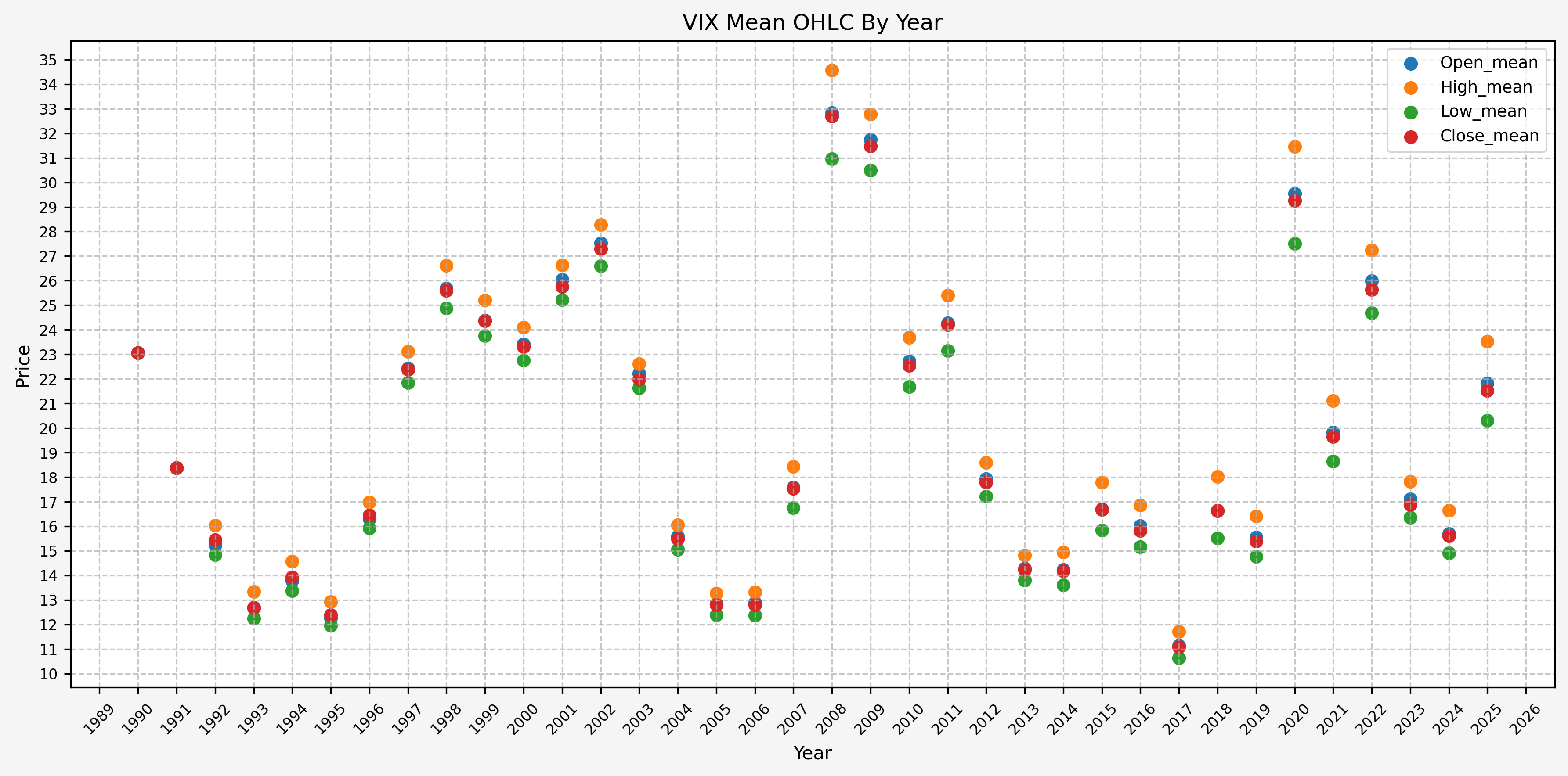
It is interesting to see how much the mean OHLC values vary by year.

And finally, we can run the statistics individually for each month:

1
2
3
4
5
6
7
8
# Group by month and calculate mean and std for OHLC
vix_stats_by_month = vix.groupby(vix.index.month)[["Open", "High", "Low", "Close"]].agg(["mean", "std"])

# Flatten the column MultiIndex
vix_stats_by_month.columns = ['_'.join(col).strip() for col in vix_stats_by_month.columns.values]
vix_stats_by_month.index.name = "Month"

display(vix_stats_by_month)

Gives us:

Month	Open_mean	Open_std	Open_min	Open_max	High_mean	High_std	High_min	High_max	Low_mean	Low_std	Low_min	Low_max	Close_mean	Close_std	Close_min	Close_max
1	19.34	7.21	9.01	51.52	20.13	7.58	9.31	57.36	18.60	6.87	8.92	49.27	19.22	7.17	9.15	56.65
2	19.67	7.22	10.19	52.50	20.51	7.65	10.26	53.16	18.90	6.81	9.70	48.97	19.58	7.13	10.02	52.62
3	20.47	9.63	10.59	82.69	21.39	10.49	11.24	85.47	19.54	8.65	10.53	70.37	20.35	9.56	10.74	82.69
4	19.43	7.48	10.39	60.13	20.24	7.93	10.89	60.59	18.65	6.88	10.22	52.76	19.29	7.28	10.36	57.06
5	18.60	6.04	9.75	47.66	19.40	6.43	10.14	48.20	17.89	5.63	9.56	40.30	18.51	5.96	9.77	45.79
6	18.45	5.80	9.79	44.09	19.15	6.07	10.28	44.44	17.73	5.44	9.37	34.97	18.34	5.72	9.75	40.79
7	17.87	5.75	9.18	48.17	18.58	5.98	9.52	48.46	17.24	5.48	8.84	42.05	17.80	5.67	9.36	44.92
8	19.17	6.74	10.04	45.34	20.12	7.45	10.32	65.73	18.44	6.38	9.52	41.77	19.18	6.87	9.93	48.00
9	20.51	8.32	9.59	48.93	21.35	8.64	9.83	49.35	19.74	7.90	9.36	43.74	20.43	8.20	9.51	46.72
10	21.83	10.28	9.23	79.13	22.83	11.10	9.62	89.53	20.93	9.51	9.11	67.80	21.75	10.24	9.19	80.06
11	20.34	9.65	9.31	80.74	21.04	10.03	9.74	81.48	19.55	9.02	8.56	72.76	20.16	9.52	9.14	80.86
12	19.34	8.26	9.36	66.68	20.09	8.53	9.55	68.60	18.63	7.88	8.89	62.31	19.29	8.16	9.31	68.51

Deciles - VIX

Here are the levels for each decile, for the full dataset:

1
2
vix_deciles = vix.quantile(np.arange(0, 1.1, 0.1))
display(vix_deciles)

Gives us:

	Close	High	Low	Open
0.00	9.14	9.31	8.56	9.01
0.10	12.12	12.63	11.72	12.13
0.20	13.26	13.88	12.85	13.31
0.30	14.61	15.29	14.08	14.68
0.40	16.10	16.76	15.56	16.13
0.50	17.66	18.39	17.08	17.70
0.60	19.55	20.39	19.00	19.69
0.70	21.64	22.65	20.99	21.79
0.80	24.31	25.36	23.50	24.38
0.90	28.70	30.00	27.78	28.86
1.00	82.69	89.53	72.76	82.69

Plots - VIX

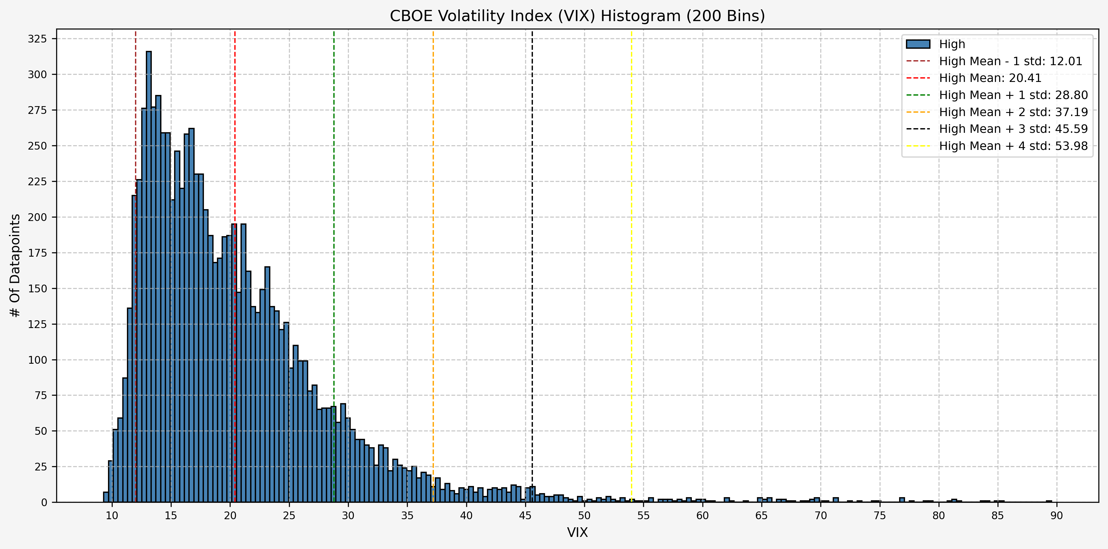
Histogram Distribution - VIX

A quick histogram gives us the distribution for the entire dataset, along with the levels for the mean minus 1 standard deviation, mean, mean plus 1 standard deviation, mean plus 2 standard deviations, mean plus 3 standard deviations, and mean plus 4 standard deviations:

Histogram, Mean, And Standard Deviations

Historical Data - VIX

Here’s two plots for the dataset. The first covers 1990 - 2009, and the second 2010 - Present. This is the daily high level:

VIX Daily High, 1990 - 2009

VIX Daily High, 2010 - Present

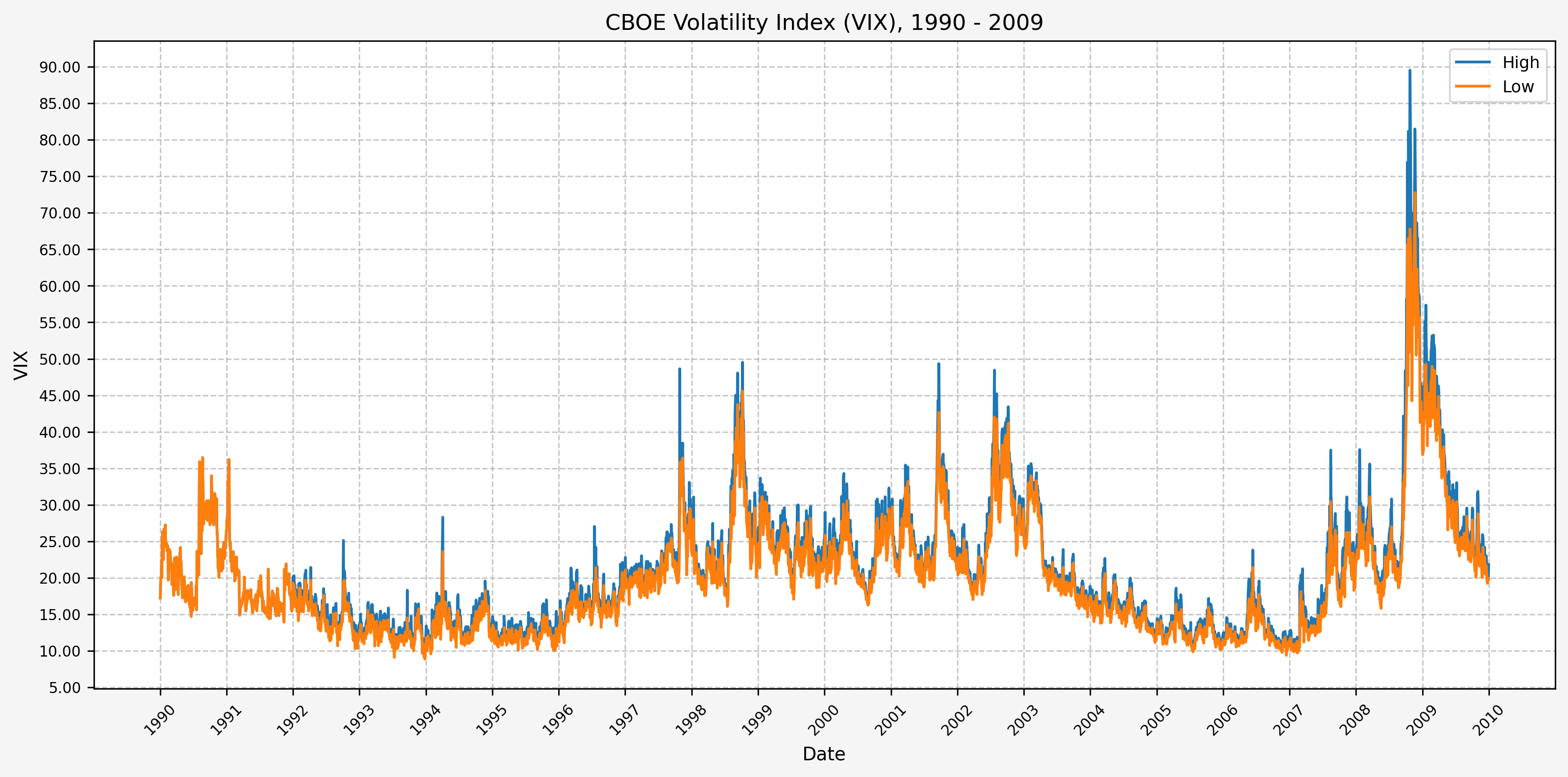
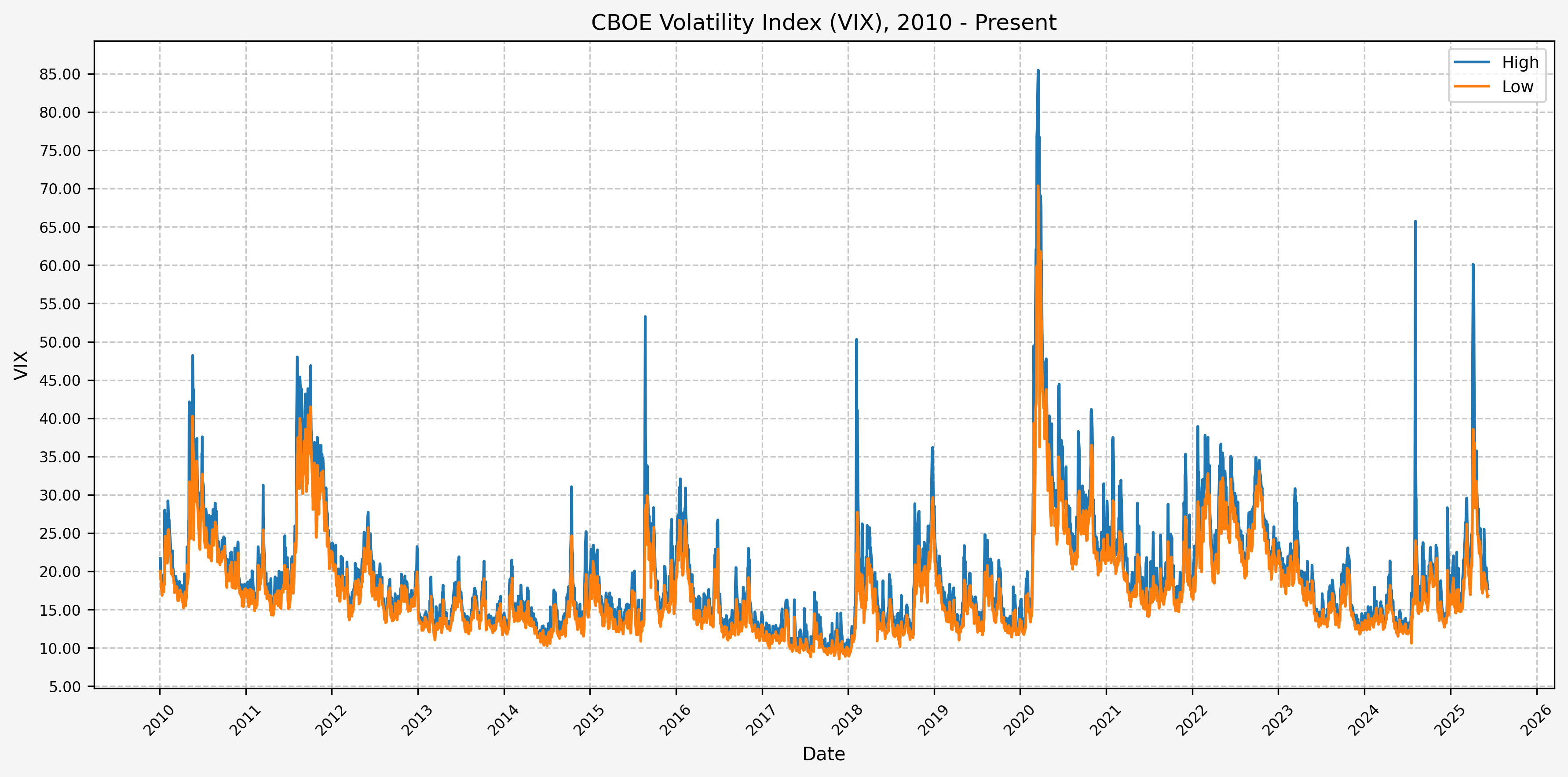
From these plots, we can see the following:

The VIX has really only jumped above 50 several times (GFC, COVID, recently in August of 2024)
The highest levels (> 80) occured only during the GFC & COVID
Interestingly, the VIX did not ever get above 50 during the .com bubble

Stats By Year - VIX

Here’s the plot for the mean OHLC values for the VIX by year:

VIX OHLC Stats By Year

Stats By Month - VIX

Here’s the plot for the mean OHLC values for the VIX by month:

VIX OHLC Stats By Month

Data Overview (VVIX)

Before moving on to generating a signal, let’s run the above data overview code again, but this time for the CBOE VVIX. From the CBOE VVIX website:

“Volatility is often called a new asset class, and every asset class deserves its own volatility index. The Cboe VVIX IndexSM represents the expected volatility of the VIX®. VVIX derives the expected 30-day volatility of VIX by applying the VIX algorithm to VIX options.”

Looking at the statistics of the VVIX should give us an idea of the volatility of the VIX.

Acquire CBOE VVIX Data

First, let’s get the data:

1
2
3
4
5
6
7
8
9
yf_pull_data(
    base_directory=DATA_DIR,
    ticker="^VVIX",
    source="Yahoo_Finance", 
    asset_class="Indices", 
    excel_export=True,
    pickle_export=True,
    output_confirmation=True,
)

Load Data - VVIX

Now that we have the data, let’s load it up and take a look:

 1
 2
 3
 4
 5
 6
 7
 8
 9
10
11
12
13
14
15
16
17
18
19
20
21
22
23
24
25
26
# Set decimal places
pandas_set_decimal_places(2)

# VVIX
vvix = load_data(
    base_directory=DATA_DIR,
    ticker="^VVIX",
    source="Yahoo_Finance", 
    asset_class="Indices",
    timeframe="Daily",
)

# Set 'Date' column as datetime
vvix['Date'] = pd.to_datetime(vvix['Date'])

# Drop 'Volume'
vvix.drop(columns = {'Volume'}, inplace = True)

# Set Date as index
vvix.set_index('Date', inplace = True)

# Check to see if there are any NaN values
vvix[vvix['High'].isna()]

# Forward fill to clean up missing data
vvix['High'] = vvix['High'].ffill()

DataFrame Info - VVIX

Now, running:

1
df_info(vvix)

Gives us the following:

 1
 2
 3
 4
 5
 6
 7
 8
 9
10
11
12
13
The columns, shape, and data types are:

<class 'pandas.core.frame.DataFrame'>
DatetimeIndex: 8925 entries, 1990-01-02 to 2025-06-09
Data columns (total 4 columns):
 #   Column  Non-Null Count  Dtype  
---  ------  --------------  -----  
 0   Close   8925 non-null   float64
 1   High    8925 non-null   float64
 2   Low     8925 non-null   float64
 3   Open    8925 non-null   float64
dtypes: float64(4)
memory usage: 348.6 KB

The first 5 rows are:

Date	Close	High	Low	Open
1990-01-02 00:00:00	17.24	17.24	17.24	17.24
1990-01-03 00:00:00	18.19	18.19	18.19	18.19
1990-01-04 00:00:00	19.22	19.22	19.22	19.22
1990-01-05 00:00:00	20.11	20.11	20.11	20.11
1990-01-08 00:00:00	20.26	20.26	20.26	20.26

The last 5 rows are:

Date	Close	High	Low	Open
2025-06-03 00:00:00	17.69	19.21	17.64	18.83
2025-06-04 00:00:00	17.61	18.07	17.41	17.68
2025-06-05 00:00:00	18.48	18.80	17.08	17.68
2025-06-06 00:00:00	16.77	18.35	16.65	18.16
2025-06-09 00:00:00	17.16	17.72	16.82	17.69

Statistics - VVIX

Here are the statistics for the VVIX, generated in the same manner as above for the VIX:

 1
 2
 3
 4
 5
 6
 7
 8
 9
10
vvix_stats = vvix.describe()
num_std = [-1, 0, 1, 2, 3, 4, 5]
for num in num_std:
    vvix_stats.loc[f"mean + {num} std"] = {
        'Open': vvix_stats.loc['mean']['Open'] + num * vvix_stats.loc['std']['Open'],
        'High': vvix_stats.loc['mean']['High'] + num * vvix_stats.loc['std']['High'],
        'Low': vvix_stats.loc['mean']['Low'] + num * vvix_stats.loc['std']['Low'],
        'Close': vvix_stats.loc['mean']['Close'] + num * vvix_stats.loc['std']['Close'],
    }
display(vvix_stats)

Gives us:

	Close	High	Low	Open
count	4629.00	4629.00	4629.00	4629.00
mean	93.50	95.55	91.94	93.75
std	16.44	18.04	15.09	16.49
min	59.74	59.74	59.31	59.31
25%	82.34	83.46	81.48	82.55
50%	90.54	92.26	89.37	90.86
75%	102.20	105.01	99.93	102.55
max	207.59	212.22	187.27	212.22
mean + -1 std	77.06	77.50	76.85	77.26
mean + 0 std	93.50	95.55	91.94	93.75
mean + 1 std	109.94	113.59	107.04	110.25
mean + 2 std	126.38	131.64	122.13	126.74
mean + 3 std	142.82	149.68	137.22	143.23
mean + 4 std	159.26	167.73	152.32	159.72
mean + 5 std	175.69	185.77	167.41	176.21

We can also run the statistics individually for each year:

1
2
3
4
5
6
7
8
# Group by year and calculate mean and std for OHLC
vvix_stats_by_year = vvix.groupby(vvix.index.year)[["Open", "High", "Low", "Close"]].agg(["mean", "std"])

# Flatten the column MultiIndex
vvix_stats_by_year.columns = ['_'.join(col).strip() for col in vvix_stats_by_year.columns.values]
vvix_stats_by_year.index.name = "Year"

display(vvix_stats_by_year)

Gives us:

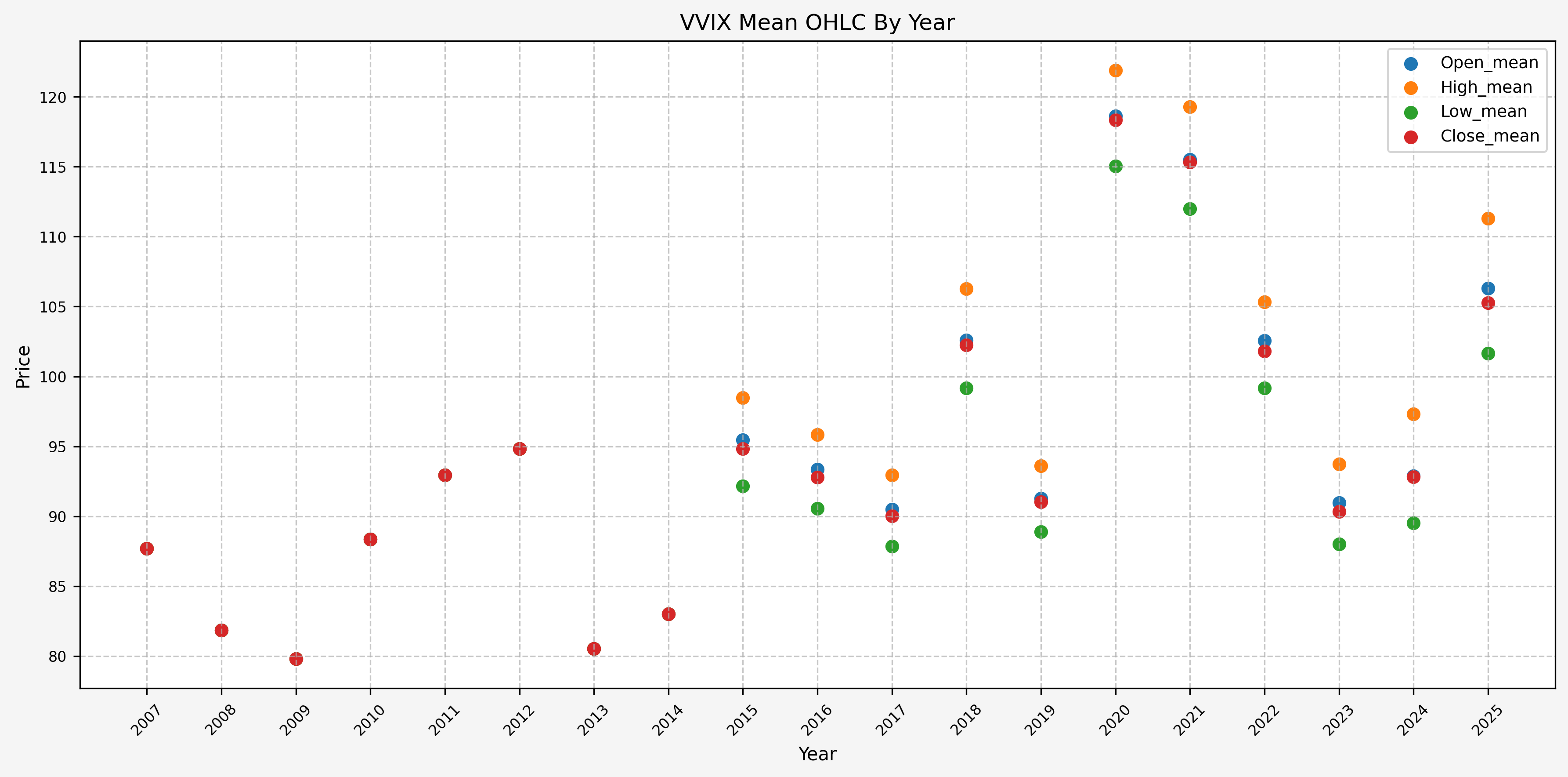
Year	Open_mean	Open_std	Open_min	Open_max	High_mean	High_std	High_min	High_max	Low_mean	Low_std	Low_min	Low_max	Close_mean	Close_std	Close_min	Close_max
2007	87.68	13.31	63.52	142.99	87.68	13.31	63.52	142.99	87.68	13.31	63.52	142.99	87.68	13.31	63.52	142.99
2008	81.85	15.60	59.74	134.87	81.85	15.60	59.74	134.87	81.85	15.60	59.74	134.87	81.85	15.60	59.74	134.87
2009	79.78	8.63	64.95	104.02	79.78	8.63	64.95	104.02	79.78	8.63	64.95	104.02	79.78	8.63	64.95	104.02
2010	88.36	13.07	64.87	145.12	88.36	13.07	64.87	145.12	88.36	13.07	64.87	145.12	88.36	13.07	64.87	145.12
2011	92.94	10.21	75.94	134.63	92.94	10.21	75.94	134.63	92.94	10.21	75.94	134.63	92.94	10.21	75.94	134.63
2012	94.84	8.38	78.42	117.44	94.84	8.38	78.42	117.44	94.84	8.38	78.42	117.44	94.84	8.38	78.42	117.44
2013	80.52	8.97	62.71	111.43	80.52	8.97	62.71	111.43	80.52	8.97	62.71	111.43	80.52	8.97	62.71	111.43
2014	83.01	14.33	61.76	138.60	83.01	14.33	61.76	138.60	83.01	14.33	61.76	138.60	83.01	14.33	61.76	138.60
2015	95.44	15.59	73.07	212.22	98.47	16.39	76.41	212.22	92.15	13.35	72.20	148.68	94.82	14.75	73.18	168.75
2016	93.36	10.02	77.96	131.95	95.82	10.86	78.86	132.42	90.54	8.99	76.17	115.15	92.80	10.07	76.17	125.13
2017	90.50	8.65	75.09	134.98	92.94	9.64	77.34	135.32	87.85	7.78	71.75	117.29	90.01	8.80	75.64	135.32
2018	102.60	13.22	83.70	176.72	106.27	16.26	85.00	203.73	99.17	11.31	82.60	165.35	102.26	14.04	83.21	180.61
2019	91.28	8.43	75.58	112.75	93.61	8.98	75.95	117.63	88.90	7.86	74.36	111.48	91.03	8.36	74.98	114.40
2020	118.64	19.32	88.39	203.03	121.91	20.88	88.54	209.76	115.05	17.37	85.31	187.27	118.36	19.39	86.87	207.59
2021	115.51	9.37	96.09	151.35	119.29	11.70	98.36	168.78	111.99	8.14	95.92	144.19	115.32	10.20	97.09	157.69
2022	102.58	18.01	76.48	161.09	105.32	19.16	77.93	172.82	99.17	16.81	76.13	153.26	101.81	17.81	77.05	154.38
2023	90.95	8.64	74.43	127.73	93.72	9.98	75.31	137.65	88.01	7.37	72.27	119.64	90.34	8.38	73.88	124.75
2024	92.88	15.06	59.31	169.68	97.32	18.33	74.79	192.49	89.51	13.16	59.31	137.05	92.81	15.60	73.26	173.32
2025	106.30	15.89	83.19	186.33	111.30	18.68	85.82	189.03	101.64	12.37	81.73	146.51	105.26	15.14	81.89	170.92

And finally, we can run the statistics individually for each month:

1
2
3
4
5
6
7
8
# Group by month and calculate mean and std for OHLC
vvix_stats_by_month = vvix.groupby(vvix.index.month)[["Open", "High", "Low", "Close"]].agg(["mean", "std"])

# Flatten the column MultiIndex
vvix_stats_by_month.columns = ['_'.join(col).strip() for col in vvix_stats_by_month.columns.values]
vvix_stats_by_month.index.name = "Year"

display(vvix_stats_by_month)

Gives us:

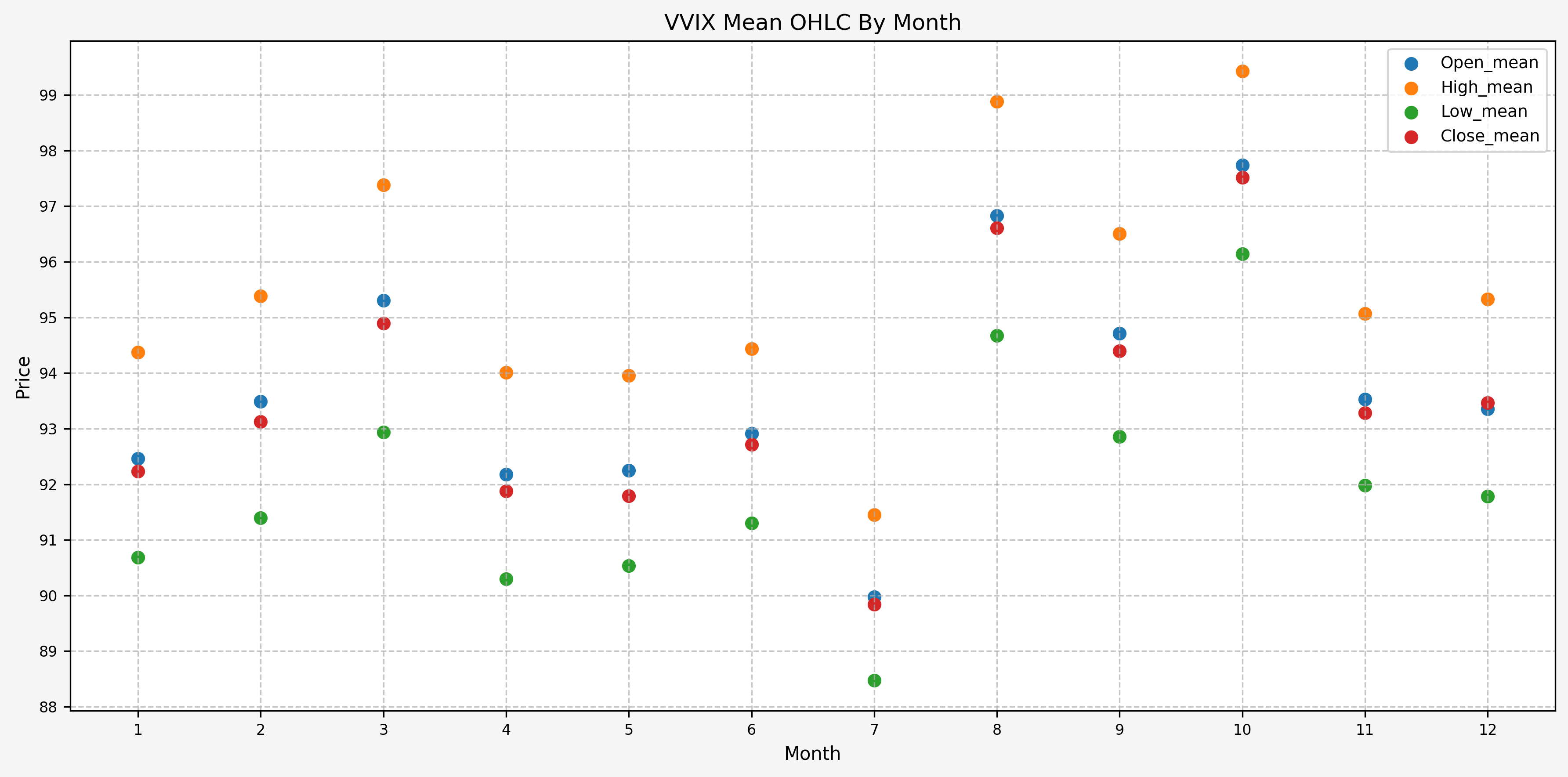
Year	Open_mean	Open_std	Open_min	Open_max	High_mean	High_std	High_min	High_max	Low_mean	Low_std	Low_min	Low_max	Close_mean	Close_std	Close_min	Close_max
1	92.46	15.63	64.87	161.09	94.37	17.63	64.87	172.82	90.69	14.23	64.87	153.26	92.23	15.78	64.87	157.69
2	93.49	18.24	65.47	176.72	95.39	20.70	65.47	203.73	91.39	16.43	65.47	165.35	93.13	18.58	65.47	180.61
3	95.30	21.66	66.97	203.03	97.38	23.56	66.97	209.76	92.94	19.51	66.97	187.27	94.89	21.59	66.97	207.59
4	92.18	19.03	59.74	186.33	94.01	20.57	59.74	189.03	90.30	17.21	59.74	152.01	91.88	18.60	59.74	170.92
5	92.25	16.93	61.76	145.18	93.95	17.99	61.76	151.50	90.54	16.14	61.76	145.12	91.79	16.79	61.76	146.28
6	92.91	14.96	63.52	155.48	94.44	16.21	63.52	172.21	91.30	13.92	63.52	140.15	92.72	14.93	63.52	151.60
7	89.97	13.16	67.21	138.42	91.46	14.23	67.21	149.60	88.48	12.26	67.21	133.82	89.84	13.12	67.21	139.54
8	96.83	16.94	68.05	212.22	98.89	18.72	68.05	212.22	94.68	14.86	68.05	148.68	96.61	16.63	68.05	173.32
9	94.71	14.03	67.94	135.17	96.50	15.52	67.94	146.31	92.86	12.50	67.94	128.46	94.40	13.78	67.94	138.93
10	97.74	14.01	64.97	149.60	99.43	15.11	64.97	154.99	96.14	13.35	64.97	144.55	97.52	14.15	64.97	152.01
11	93.53	14.17	63.77	142.68	95.07	15.36	63.77	161.76	91.98	13.39	63.77	140.44	93.28	14.24	63.77	149.74
12	93.35	15.03	59.31	151.35	95.33	16.63	62.71	168.37	91.78	13.70	59.31	144.19	93.46	15.07	62.71	156.10

Deciles - VVIX

Here are the levels for each decile, for the full dataset:

1
2
vvix_deciles = vvix.quantile(np.arange(0, 1.1, 0.1))
display(vvix_deciles)

Gives us:

	Close	High	Low	Open
0.00	59.74	59.74	59.31	59.31
0.10	75.83	76.02	75.44	75.80
0.20	80.58	81.43	79.82	80.75
0.30	83.90	85.22	83.01	84.17
0.40	87.08	88.57	85.98	87.46
0.50	90.54	92.26	89.37	90.86
0.60	94.21	96.14	93.03	94.51
0.70	99.11	101.53	97.43	99.40
0.80	106.06	109.40	103.90	106.48
0.90	115.27	118.80	112.48	115.53
1.00	207.59	212.22	187.27	212.22

Plots - VVIX

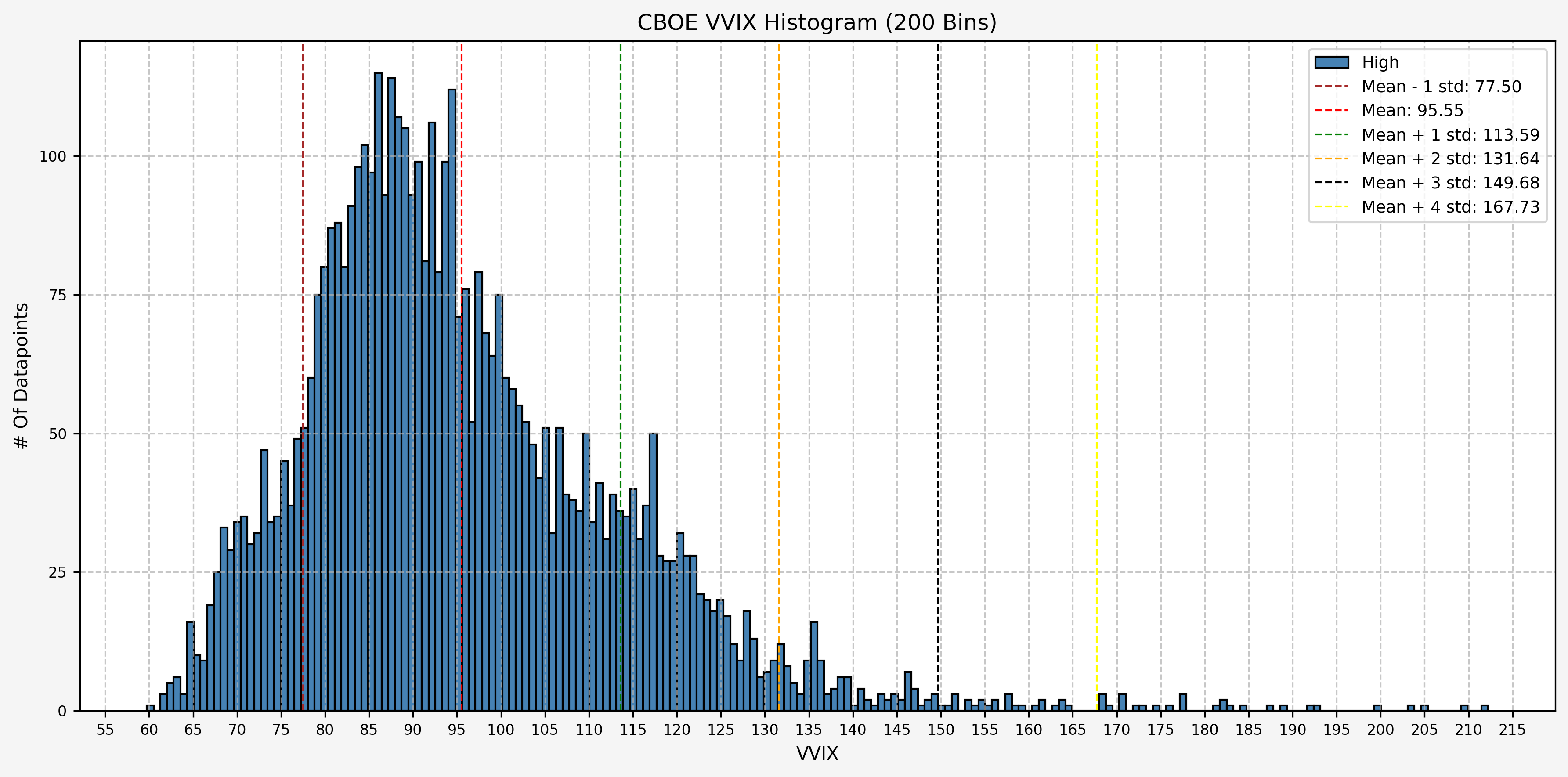
Histogram Distribution - VVIX

Histogram, Mean, And Standard Deviations

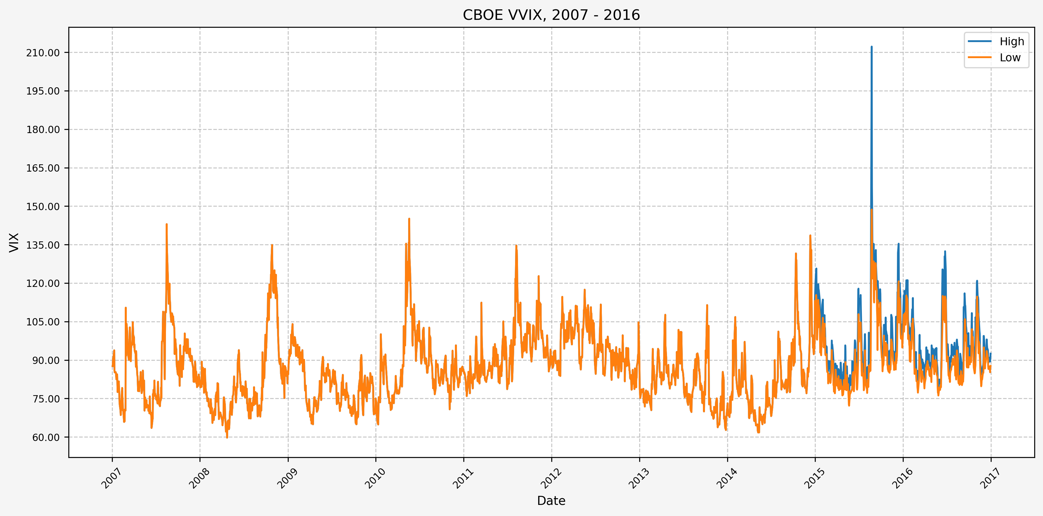
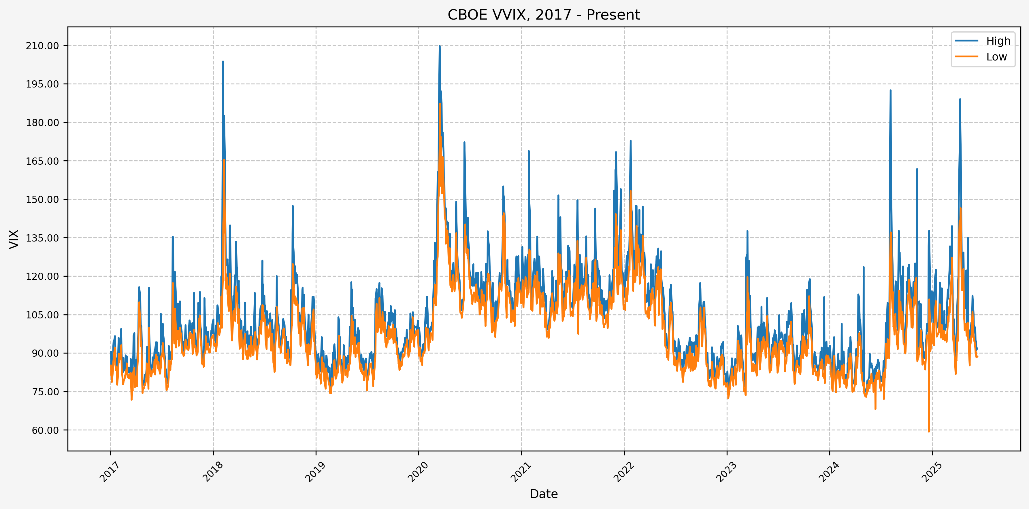
Historical Data - VVIX

Here’s two plots for the dataset. The first covers 2007 - 2016, and the second 2017 - Present. This is the daily high level:

VVIX Daily High, 2007 - 2016

VVIX Daily High, 2017 - Present

Stats By Year - VVIX

Here’s the plot for the mean OHLC values for the VVIX by year:

VVIX OHLC Stats By Year

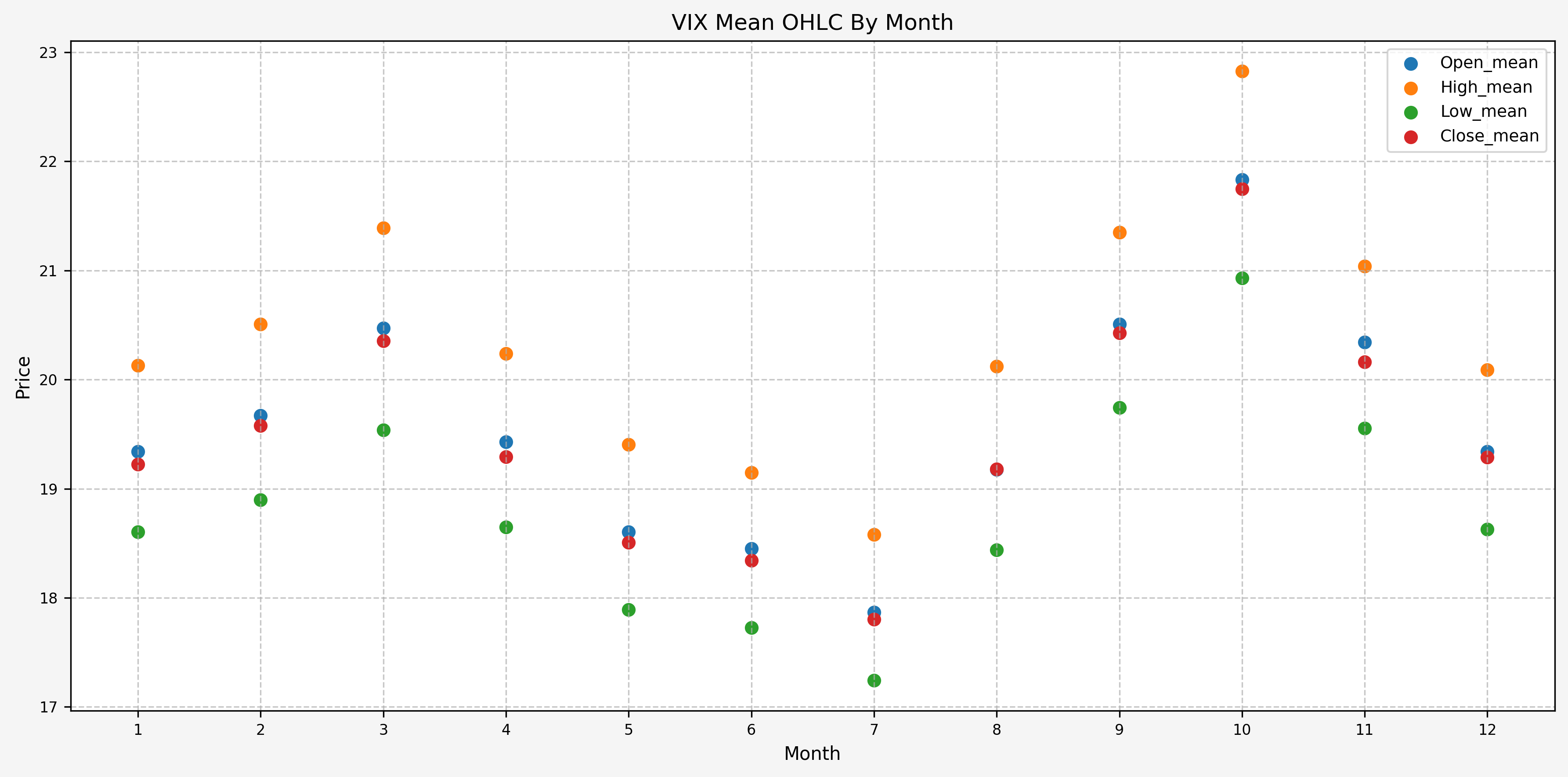
Stats By Month - VVIX

Here’s the plot for the mean OHLC values for the VVIX by month:

VVIX OHLC Stats By Month

References

Code

The jupyter notebook with the functions and all other code is available here.
The html export of the jupyter notebook is available here.
The pdf export of the jupyter notebook is available here.