Post Updates
Update 4/8/2025: Added plot for signals for each year. VIX data through 4/7/25.Update 4/9/2025: VIX data through 4/8/25.Update 4/12/2025: VIX data through 4/10/25.Update 4/22/2025: VIX data through 4/18/25.Update 4/23/2025: VIX data through 4/22/25.Update 4/25/2025: VIX data through 4/23/25. Added section for trade history, including open and closed positions.Update 4/28/2025: VIX data through 4/25/25.
Introduction
From the CBOE VIX website:
“Cboe Global Markets revolutionized investing with the creation of the Cboe Volatility Index® (VIX® Index), the first benchmark index to measure the market’s expectation of future volatility. The VIX Index is based on options of the S&P 500® Index, considered the leading indicator of the broad U.S. stock market. The VIX Index is recognized as the world’s premier gauge of U.S. equity market volatility.”
In this tutorial, we will investigate finding a signal to use as a basis to trade the VIX.
VIX Data
I don’t have access to data for the VIX through Nasdaq Data Link, but for our purposes Yahoo Finance is sufficient.
Using the yfinance python module, we can pull what we need and quicky dump it to excel to retain it for future use.
Python Functions
Typical Functions
First, the typical set of functions I use:
 1
 2
 3
 4
 5
 6
 7
 8
 9
10
11
12
13
14
15
16
17
18
19
20
21
22
23
24
25
26
27
28
29
30
31
32
33
34
35
36
37
38
39
| from pathlib import Path
def export_track_md_deps(
dep_file: Path,
md_filename: str,
content: str,
) -> None:
"""
Export Markdown content to a file and track it as a dependency.
This function writes the provided content to the specified Markdown file and
appends the filename to the given dependency file (typically `index_dep.txt`).
This is useful in workflows where Markdown fragments are later assembled
into a larger document (e.g., a Hugo `index.md`).
Parameters:
-----------
dep_file : Path
Path to the dependency file that tracks Markdown fragment filenames.
md_filename : str
The name of the Markdown file to export.
content : str
The Markdown-formatted content to write to the file.
Returns:
--------
None
Example:
--------
>>> export_track_md_deps(Path("index_dep.txt"), "01_intro.md", "# Introduction\n...")
✅ Exported and tracked: 01_intro.md
"""
Path(md_filename).write_text(content)
with dep_file.open("a") as f:
f.write(md_filename + "\n")
print(f"✅ Exported and tracked: {md_filename}")
|
 1
 2
 3
 4
 5
 6
 7
 8
 9
10
11
12
13
14
15
16
17
18
19
20
21
22
23
24
25
26
27
28
29
30
31
32
33
34
| from IPython.display import display
def df_info(df) -> None:
"""
Display summary information about a pandas DataFrame.
This function prints:
- The DataFrame's column names, shape, and data types via `df.info()`
- The first 5 rows using `df.head()`
- The last 5 rows using `df.tail()`
It uses `display()` for better output formatting in environments like Jupyter notebooks.
Parameters:
-----------
df : pd.DataFrame
The DataFrame to inspect.
Returns:
--------
None
Example:
--------
>>> df_info(my_dataframe)
"""
print("The columns, shape, and data types are:")
print(df.info())
print("The first 5 rows are:")
display(df.head())
print("The last 5 rows are:")
display(df.tail())
|
 1
 2
 3
 4
 5
 6
 7
 8
 9
10
11
12
13
14
15
16
17
18
19
20
21
22
23
24
25
26
27
28
29
30
31
32
33
34
35
36
37
38
39
40
41
42
43
44
45
46
47
48
49
50
51
52
53
54
55
56
57
58
59
60
61
| import io
import pandas as pd
def df_info_markdown(df: pd.DataFrame) -> str:
"""
Generate a Markdown-formatted summary of a pandas DataFrame.
This function captures and formats the output of `df.info()`, `df.head()`,
and `df.tail()` in Markdown for easy inclusion in reports, documentation,
or web-based rendering (e.g., Hugo or Jupyter export workflows).
Parameters:
-----------
df : pd.DataFrame
The DataFrame to summarize.
Returns:
--------
str
A string containing the DataFrame's info, head, and tail
formatted in Markdown.
Example:
--------
>>> print(df_info_markdown(df))
```text
The columns, shape, and data types are:
<output from df.info()>
```
The first 5 rows are:
| | col1 | col2 |
|---|------|------|
| 0 | ... | ... |
The last 5 rows are:
...
"""
buffer = io.StringIO()
# Capture df.info() output
df.info(buf=buffer)
info_str = buffer.getvalue()
# Convert head and tail to Markdown
head_str = df.head().to_markdown()
tail_str = df.tail().to_markdown()
markdown = [
"```text",
"The columns, shape, and data types are:\n",
info_str,
"```",
"\nThe first 5 rows are:\n",
head_str,
"\nThe last 5 rows are:\n",
tail_str
]
return "\n".join(markdown)
|
 1
 2
 3
 4
 5
 6
 7
 8
 9
10
11
12
13
14
15
16
17
18
19
20
21
| import pandas as pd
def pandas_set_decimal_places(decimal_places: int) -> None:
"""
Set the number of decimal places displayed for floating-point numbers in pandas.
Parameters:
----------
decimal_places : int
The number of decimal places to display for float values in pandas DataFrames and Series.
Example:
--------
>>> dp(3)
>>> pd.DataFrame([1.23456789])
0
0 1.235
"""
pd.set_option('display.float_format', lambda x: f'%.{decimal_places}f' % x)
|
 1
 2
 3
 4
 5
 6
 7
 8
 9
10
11
12
13
14
15
16
17
18
19
20
21
22
23
24
25
26
27
28
29
30
31
32
33
34
35
36
37
38
39
40
41
42
43
44
45
46
47
48
49
50
51
52
53
54
55
56
57
58
59
60
61
62
63
64
65
| import pandas as pd
from pathlib import Path
def load_data(
base_directory: str,
ticker: str,
source: str,
asset_class: str,
timeframe: str,
) -> pd.DataFrame:
"""
Load data from a CSV or Excel file into a pandas DataFrame.
This function attempts to read a file first as a CSV, then as an Excel file
(specifically looking for a sheet named 'data' and using the 'calamine' engine).
If both attempts fail, a ValueError is raised.
Parameters:
-----------
base_directory : str
Root path to read data file.
ticker : str
Ticker symbol to read.
source : str
Name of the data source (e.g., 'Yahoo').
asset_class : str
Asset class name (e.g., 'Equities').
timeframe : str
Timeframe for the data (e.g., 'Daily', 'Month_End').
Returns:
--------
pd.DataFrame
The loaded data.
Raises:
-------
ValueError
If the file could not be loaded as either CSV or Excel.
Example:
--------
>>> df = load_data(DATA_DIR, "^VIX", "Yahoo_Finance", "Indices")
"""
# Build file paths using pathlib
csv_path = Path(base_directory) / source / asset_class / timeframe / f"{ticker}.csv"
xlsx_path = Path(base_directory) / source / asset_class / timeframe / f"{ticker}.xlsx"
# Try CSV
try:
df = pd.read_csv(csv_path)
return df
except Exception:
pass
# Try Excel
try:
df = pd.read_excel(xlsx_path)
return df
except Exception:
pass
raise ValueError(f"❌ Unable to load file: {ticker}. Ensure it's a valid CSV or Excel file with a 'data' sheet.")
|
Project Specific Functions
Here’s the code for the function to pull the VIX data and export to Excel:
 1
 2
 3
 4
 5
 6
 7
 8
 9
10
11
12
13
14
15
16
17
18
19
20
21
22
23
24
25
26
27
28
29
30
31
32
33
34
35
36
37
38
39
40
41
42
43
44
45
46
47
48
49
50
51
52
53
54
55
56
57
58
59
60
61
62
63
64
65
66
67
68
69
70
71
72
73
74
75
76
77
78
79
80
| import yfinance as yf
import os
from IPython.display import display
def yf_pull_data(
base_directory: str,
ticker: str,
source: str,
asset_class: str,
excel_export: bool,
pickle_export: bool,
) -> None:
"""
Download daily price data from Yahoo Finance and export it.
Parameters:
-----------
base_directory : str
Root path to store downloaded data.
ticker : str
Ticker symbol to download.
source : str
Name of the data source (e.g., 'Yahoo').
asset_class : str
Asset class name (e.g., 'Equities').
excel_export : bool
If True, export data to Excel format.
pickle_export : bool
If True, export data to Pickle format.
Returns:
--------
None
"""
# Download data from YF
df = yf.download(ticker)
# Drop the column level with the ticker symbol
df.columns = df.columns.droplevel(1)
# Reset index
df = df.reset_index()
# Remove the "Price" header from the index
df.columns.name = None
# Reset date column
df['Date'] = df['Date'].dt.tz_localize(None)
# Set 'Date' column as index
df = df.set_index('Date', drop=True)
# Drop data from last day because it's not accrate until end of day
df = df.drop(df.index[-1])
# Create directory
directory = f"{base_directory}/{source}/{asset_class}/Daily"
os.makedirs(directory, exist_ok=True)
# Export to excel
if excel_export == True:
df.to_excel(f"{directory}/{ticker}.xlsx", sheet_name="data")
else:
pass
# Export to pickle
if pickle_export == True:
df.to_pickle(f"{directory}/{ticker}.pkl")
else:
pass
# Print confirmation and display the first and last date
# of data
print(f"The first and last date of data for {ticker} is: ")
display(df[:1])
display(df[-1:])
print(f"Yahoo Finance data complete for {ticker}")
return print(f"--------------------")
|
Data Overview
Acquire CBOE Volatility Index (VIX) Data
First, let’s get the data:
1
| yf_data_updater('^VIX')
|
Set Decimal Places
Let’s set the number of decimal places to something sane (like 2):
1
| pandas_set_decimal_places(2)
|
Load Data
Now that we have the data, let’s load it up and take a look:
 1
 2
 3
 4
 5
 6
 7
 8
 9
10
11
| # VIX
vix = load_data('^VIX.xlsx')
# Set 'Date' column as datetime
vix['Date'] = pd.to_datetime(vix['Date'])
# Drop 'Volume'
vix.drop(columns = {'Volume'}, inplace = True)
# Set Date as index
vix.set_index('Date', inplace = True)
|
Check For Missing Values & Forward Fill Any Missing Values
1
2
3
4
5
| # Check to see if there are any NaN values
vix[vix['High'].isna()]
# Forward fill to clean up missing data
vix['High'] = vix['High'].ffill()
|
VIX DataFrame Info
Now, running:
Gives us the following:
 1
 2
 3
 4
 5
 6
 7
 8
 9
10
11
12
13
| The columns, shape, and data types are:
<class 'pandas.core.frame.DataFrame'>
DatetimeIndex: 8895 entries, 1990-01-02 to 2025-04-25
Data columns (total 4 columns):
# Column Non-Null Count Dtype
--- ------ -------------- -----
0 Close 8895 non-null float64
1 High 8895 non-null float64
2 Low 8895 non-null float64
3 Open 8895 non-null float64
dtypes: float64(4)
memory usage: 347.5 KB
|
The first 5 rows are:
| Date | Close | High | Low | Open |
|---|
| 1990-01-02 00:00:00 | 17.24 | 17.24 | 17.24 | 17.24 |
| 1990-01-03 00:00:00 | 18.19 | 18.19 | 18.19 | 18.19 |
| 1990-01-04 00:00:00 | 19.22 | 19.22 | 19.22 | 19.22 |
| 1990-01-05 00:00:00 | 20.11 | 20.11 | 20.11 | 20.11 |
| 1990-01-08 00:00:00 | 20.26 | 20.26 | 20.26 | 20.26 |
The last 5 rows are:
| Date | Close | High | Low | Open |
|---|
| 2025-04-21 00:00:00 | 33.82 | 35.75 | 31.79 | 32.75 |
| 2025-04-22 00:00:00 | 30.57 | 32.68 | 30.08 | 32.61 |
| 2025-04-23 00:00:00 | 28.45 | 30.29 | 27.11 | 28.75 |
| 2025-04-24 00:00:00 | 26.47 | 29.66 | 26.36 | 28.69 |
| 2025-04-25 00:00:00 | 24.84 | 27.20 | 24.84 | 26.22 |
Statistics
Some interesting statistics jump out at us when we look at the mean, standard deviation, minimum, and maximum values. The following code:
1
2
3
4
5
6
7
8
9
| vix_stats = vix.describe()
num_std = [-1, 0, 1, 2, 3, 4, 5]
for num in num_std:
vix_stats.loc[f"mean + {num} std"] = {
'Open': vix_stats.loc['mean']['Open'] + num * vix_stats.loc['std']['Open'],
'High': vix_stats.loc['mean']['High'] + num * vix_stats.loc['std']['High'],
'Low': vix_stats.loc['mean']['Low'] + num * vix_stats.loc['std']['Low'],
'Close': vix_stats.loc['mean']['Close'] + num * vix_stats.loc['std']['Close'],
}
|
Gives us:
| Close | High | Low | Open |
|---|
| count | 8895.00 | 8895.00 | 8895.00 | 8895.00 |
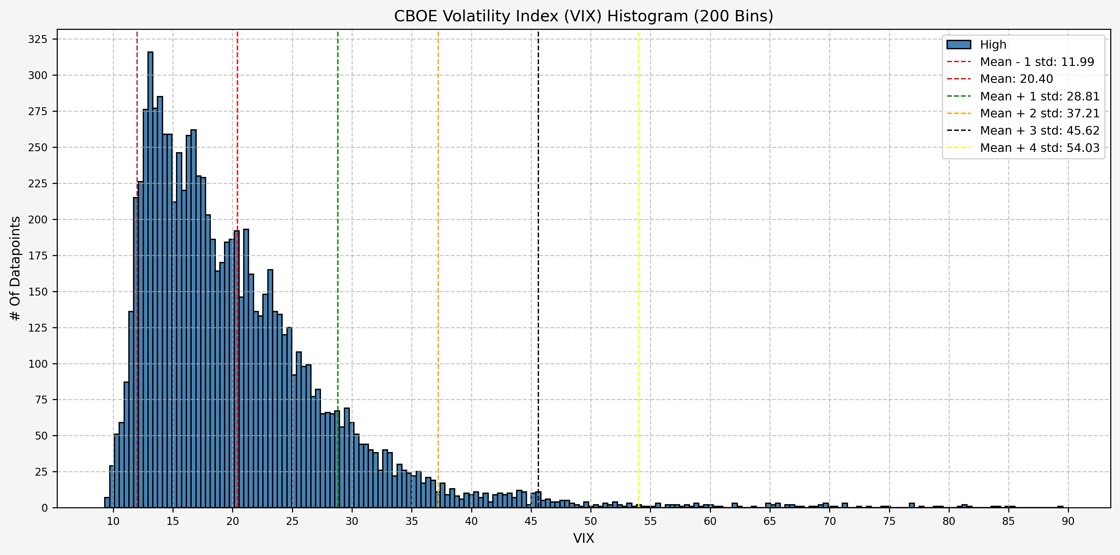
| mean | 19.49 | 20.40 | 18.82 | 19.58 |
| std | 7.85 | 8.41 | 7.40 | 7.92 |
| min | 9.14 | 9.31 | 8.56 | 9.01 |
| 25% | 13.86 | 14.53 | 13.40 | 13.93 |
| 50% | 17.64 | 18.35 | 17.06 | 17.68 |
| 75% | 22.84 | 23.83 | 22.14 | 22.97 |
| max | 82.69 | 89.53 | 72.76 | 82.69 |
| mean + -1 std | 11.65 | 11.99 | 11.42 | 11.66 |
| mean + 0 std | 19.49 | 20.40 | 18.82 | 19.58 |
| mean + 1 std | 27.34 | 28.81 | 26.22 | 27.51 |
| mean + 2 std | 35.19 | 37.21 | 33.62 | 35.43 |
| mean + 3 std | 43.03 | 45.62 | 41.02 | 43.35 |
| mean + 4 std | 50.88 | 54.03 | 48.42 | 51.27 |
| mean + 5 std | 58.73 | 62.43 | 55.82 | 59.20 |
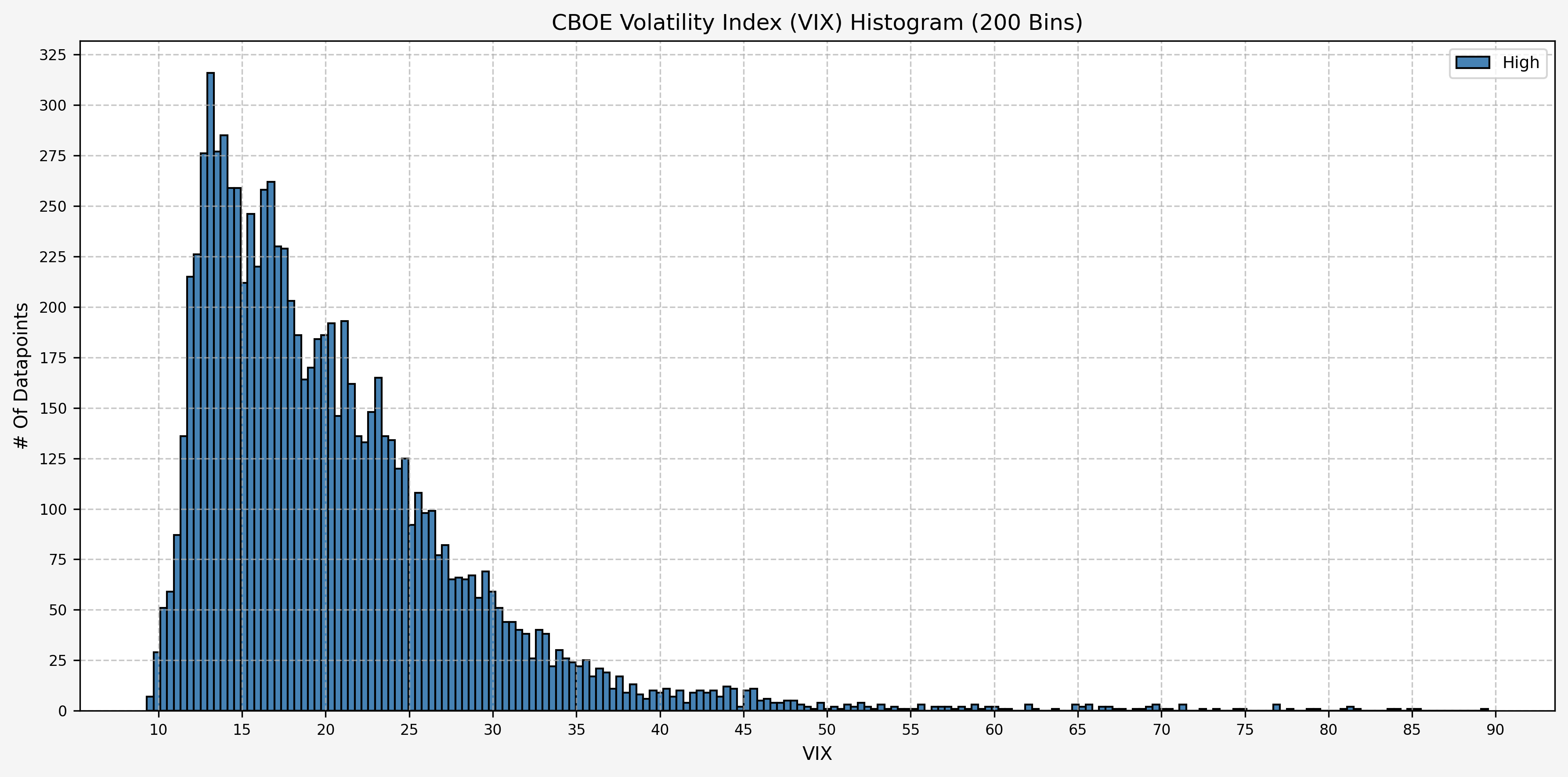
Deciles
And the levels for each decile:
1
2
| vix_deciles = vix.quantile(np.arange(0, 1.1, 0.1))
display(vix_deciles)
|
Gives us:
| Close | High | Low | Open |
|---|
| 0.00 | 9.14 | 9.31 | 8.56 | 9.01 |
| 0.10 | 12.12 | 12.62 | 11.72 | 12.13 |
| 0.20 | 13.24 | 13.87 | 12.85 | 13.30 |
| 0.30 | 14.59 | 15.28 | 14.07 | 14.67 |
| 0.40 | 16.09 | 16.75 | 15.55 | 16.12 |
| 0.50 | 17.64 | 18.35 | 17.06 | 17.68 |
| 0.60 | 19.55 | 20.38 | 19.00 | 19.68 |
| 0.70 | 21.64 | 22.64 | 20.99 | 21.79 |
| 0.80 | 24.32 | 25.36 | 23.51 | 24.39 |
| 0.90 | 28.73 | 30.02 | 27.80 | 28.88 |
| 1.00 | 82.69 | 89.53 | 72.76 | 82.69 |
Histogram Distribution
A quick histogram gives us the distribution for the entire dataset:
Now, let’s add the levels for the mean, mean plus 1 standard deviation, mean minus 1 standard deviation, and mean plus 2 standard deviations:
Plots
Historical VIX Data
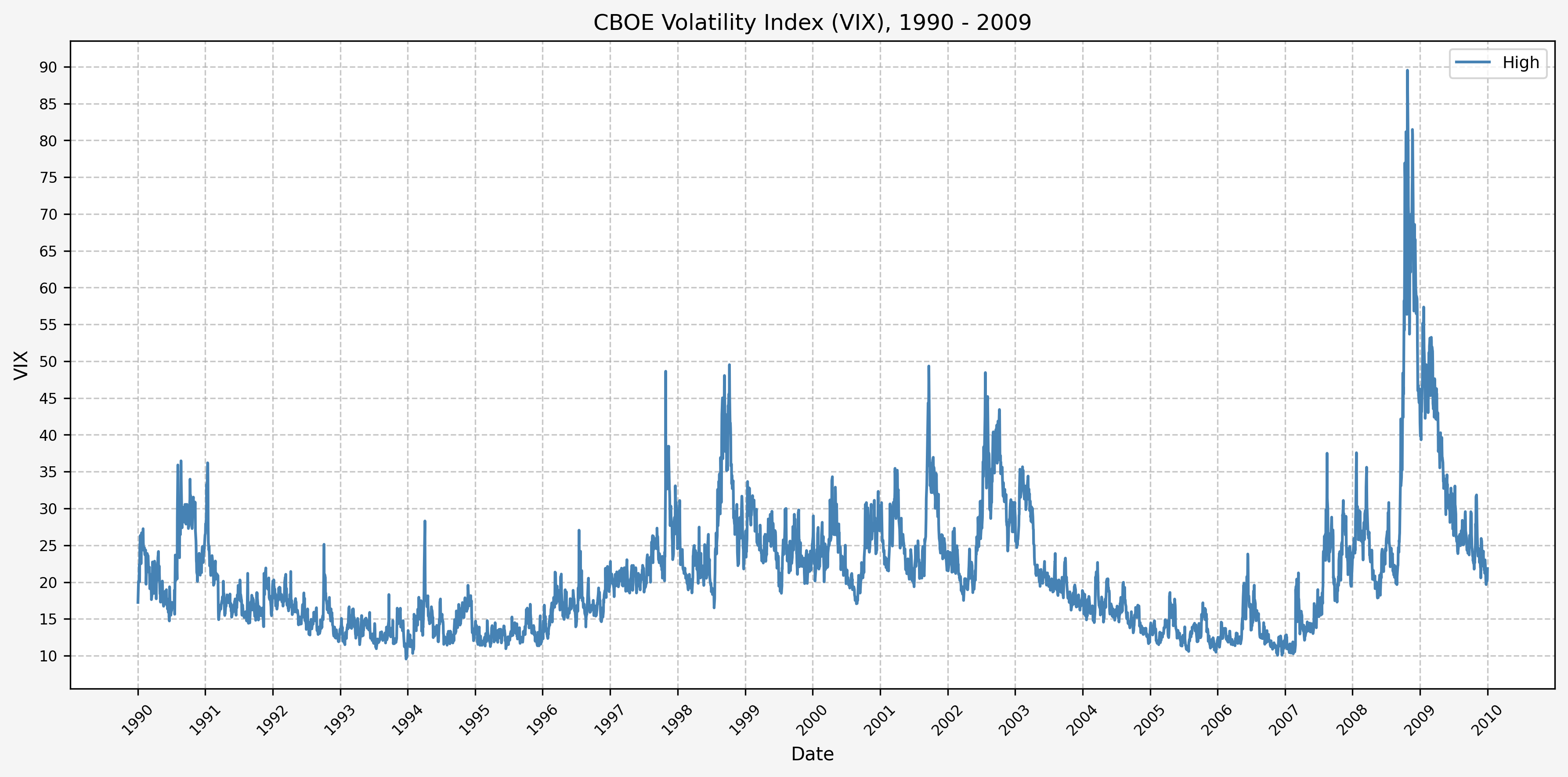
Here’s two plots for the dataset. The first covers 1990 - 2009, and the second 2010 - 2024. This is the daily high level:
1990 - 2009
2010 - Present
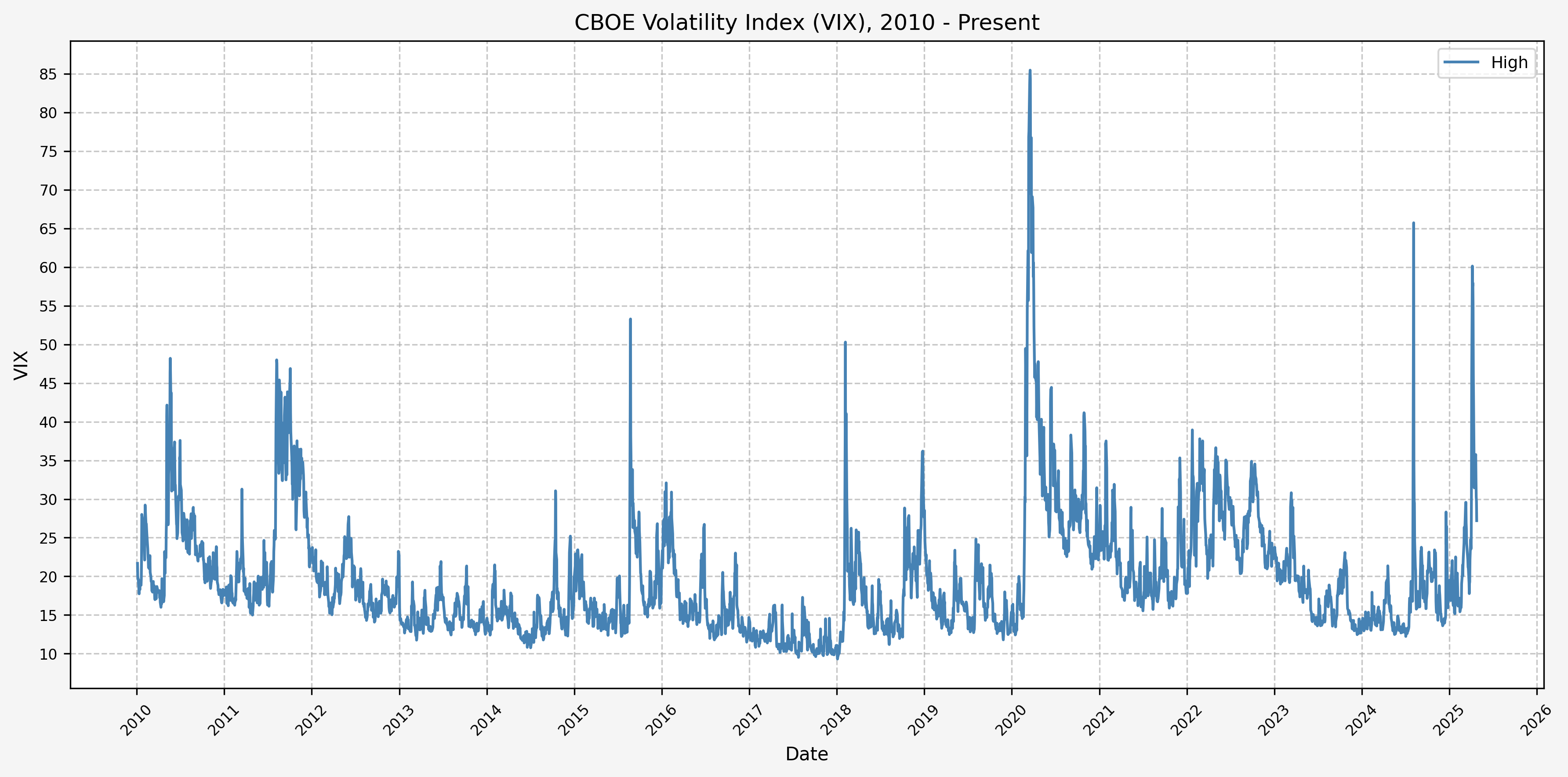
From these plots, we can see the following:
- The VIX has really only jumped above 50 several times (GFC, COVID, recently in August of 2024)
- The highest levels (> 80) occured only during the GFC & COVID
- Interestingly, the VIX did not ever get above 50 during the .com bubble
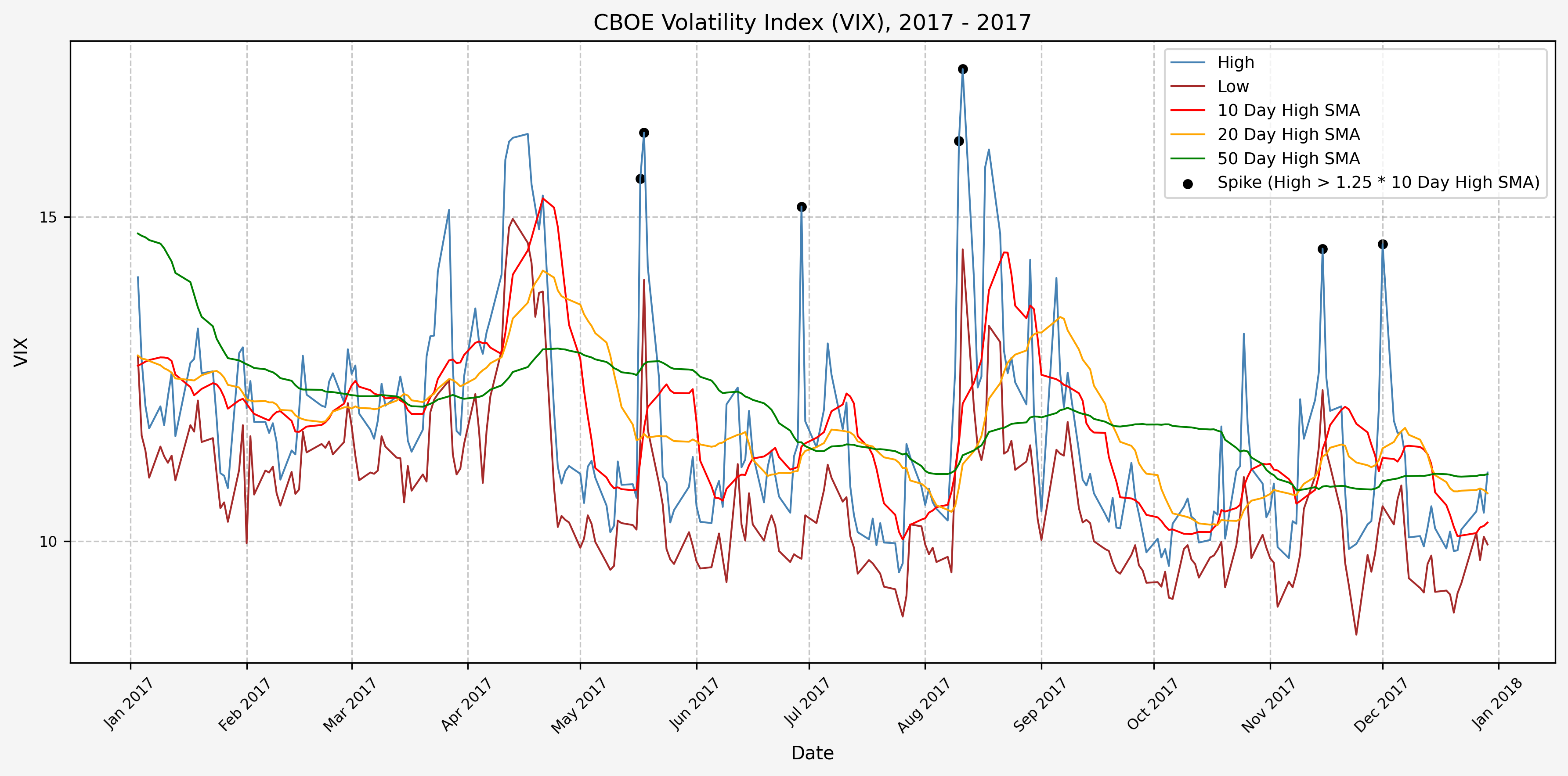
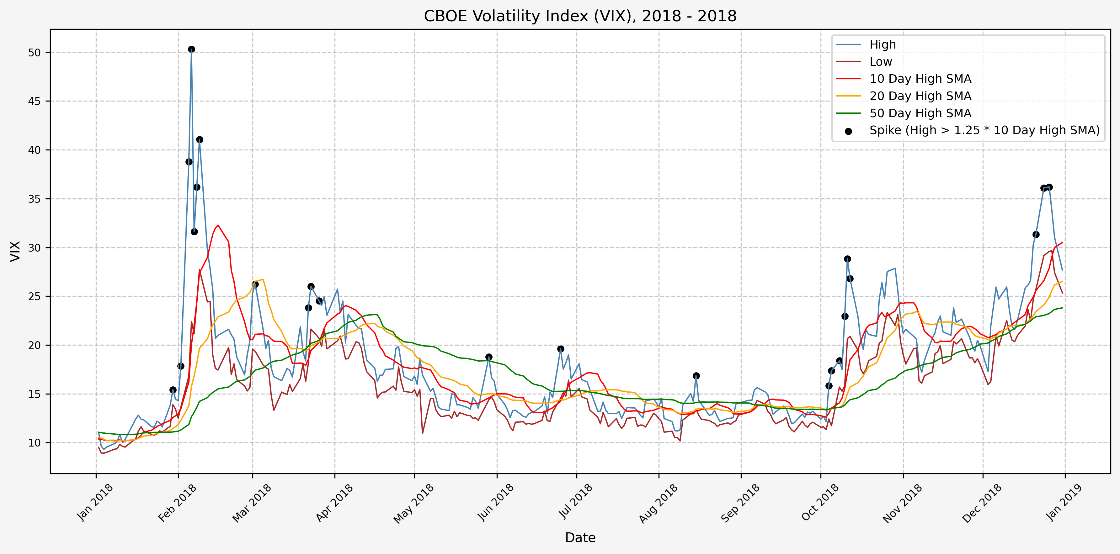
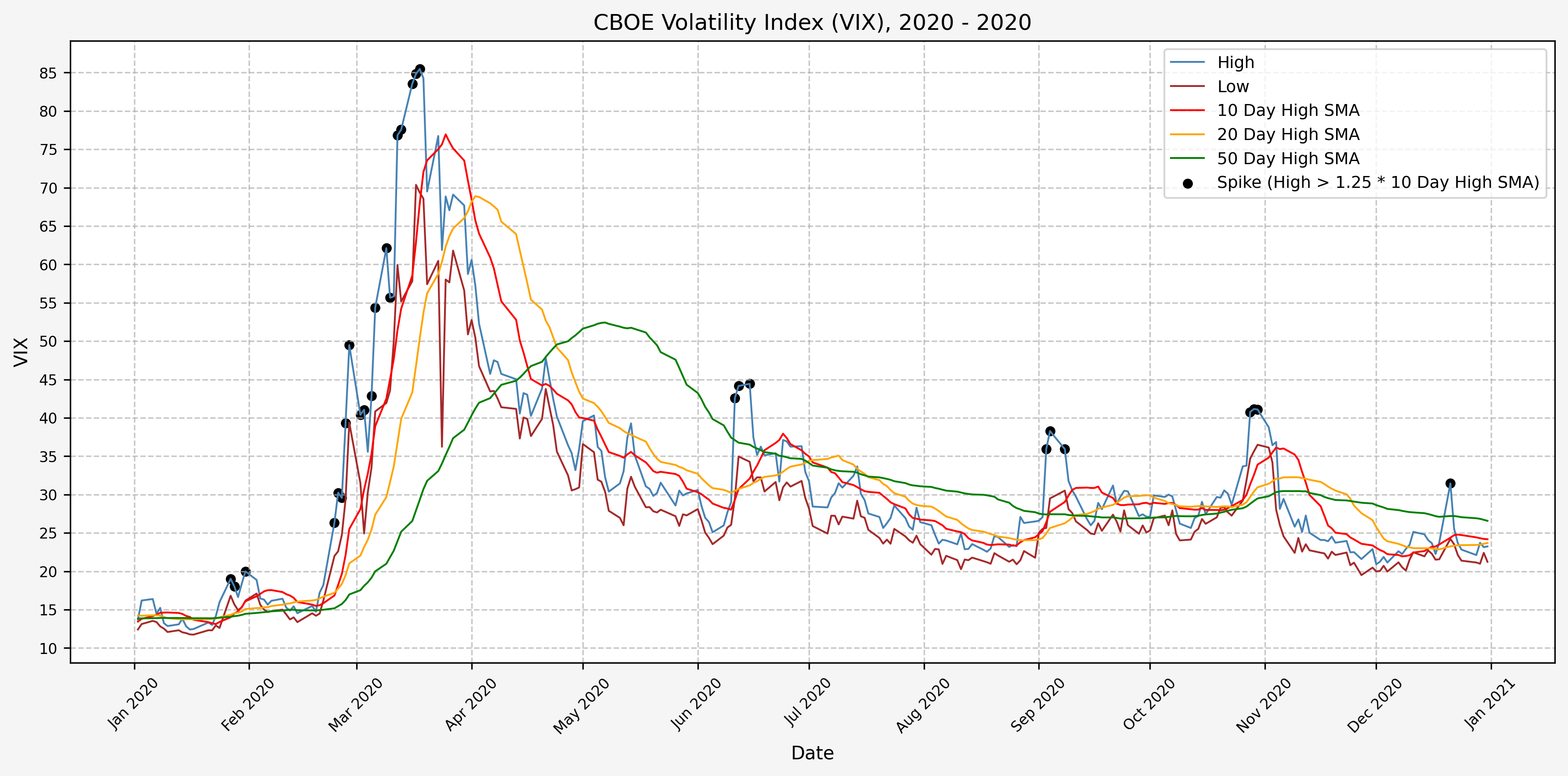
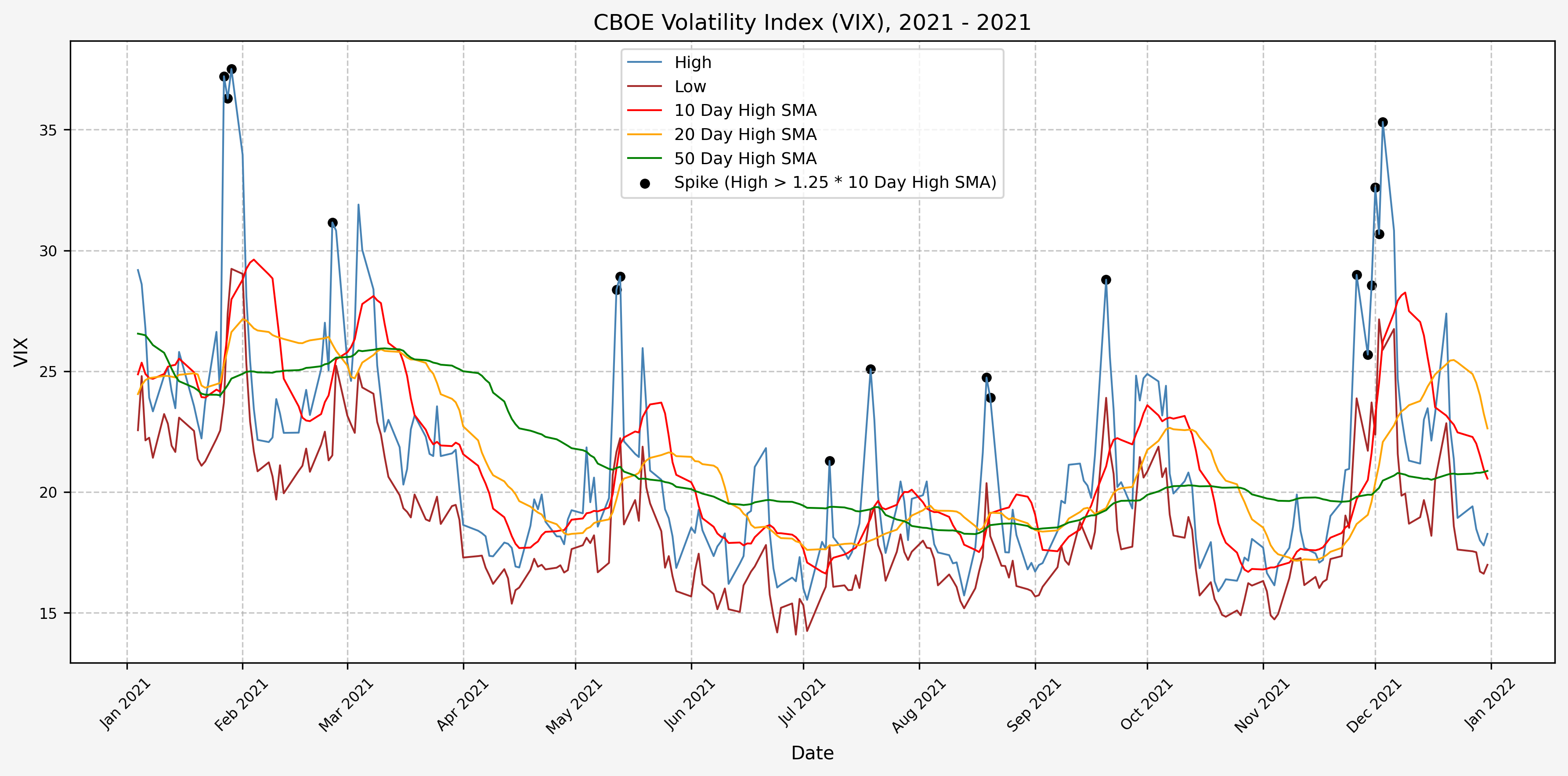
Investigating A Signal
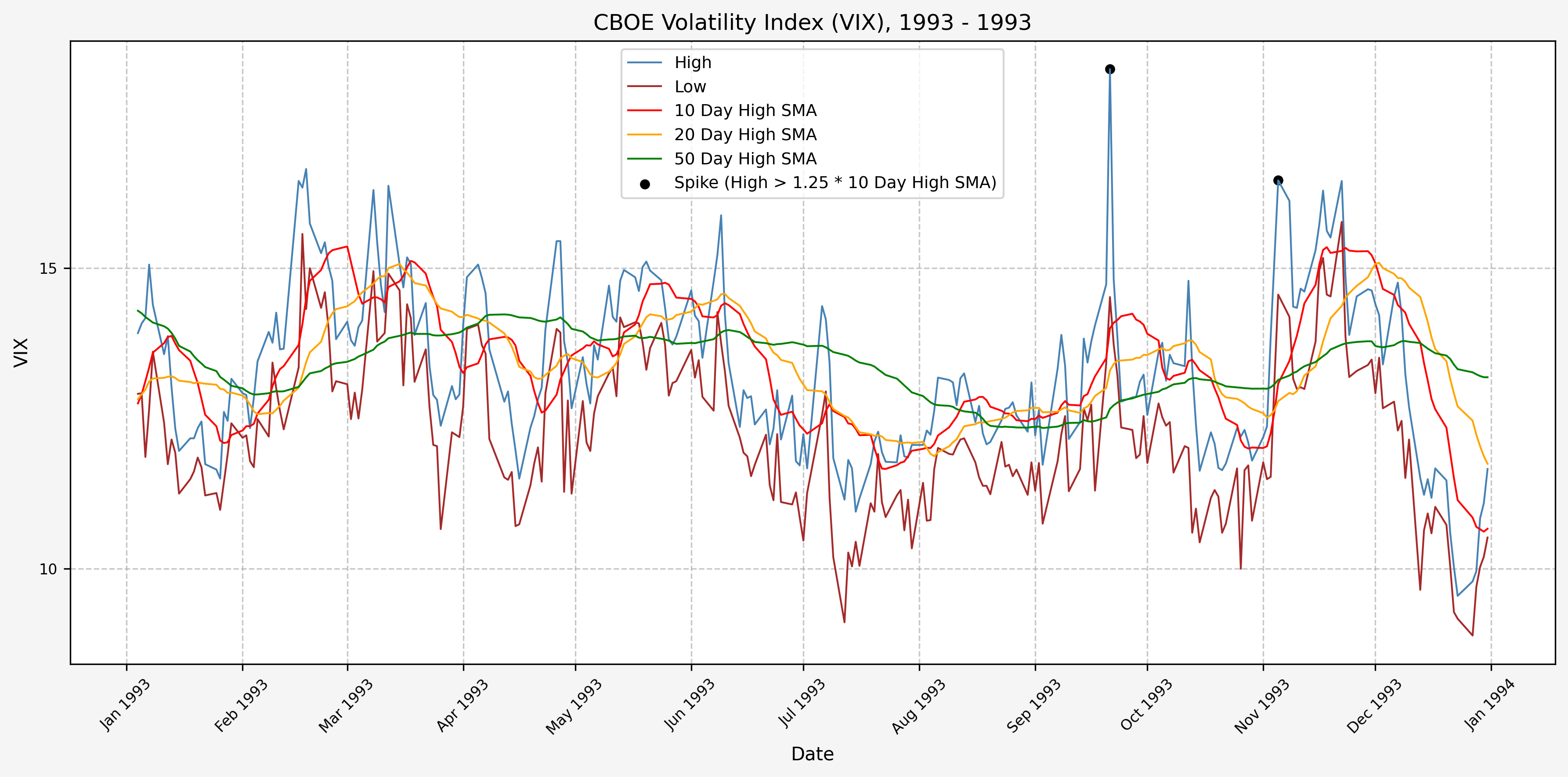
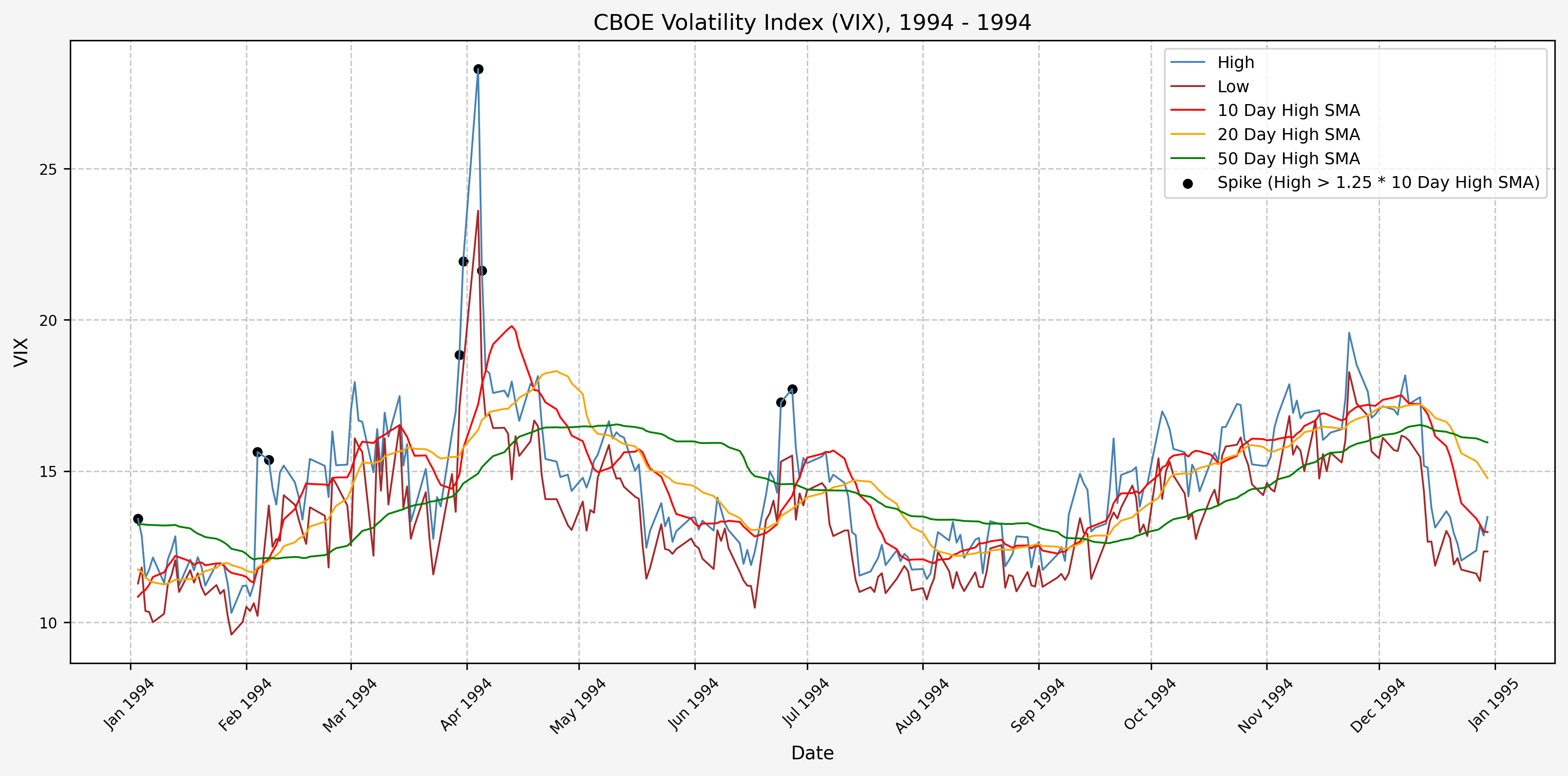
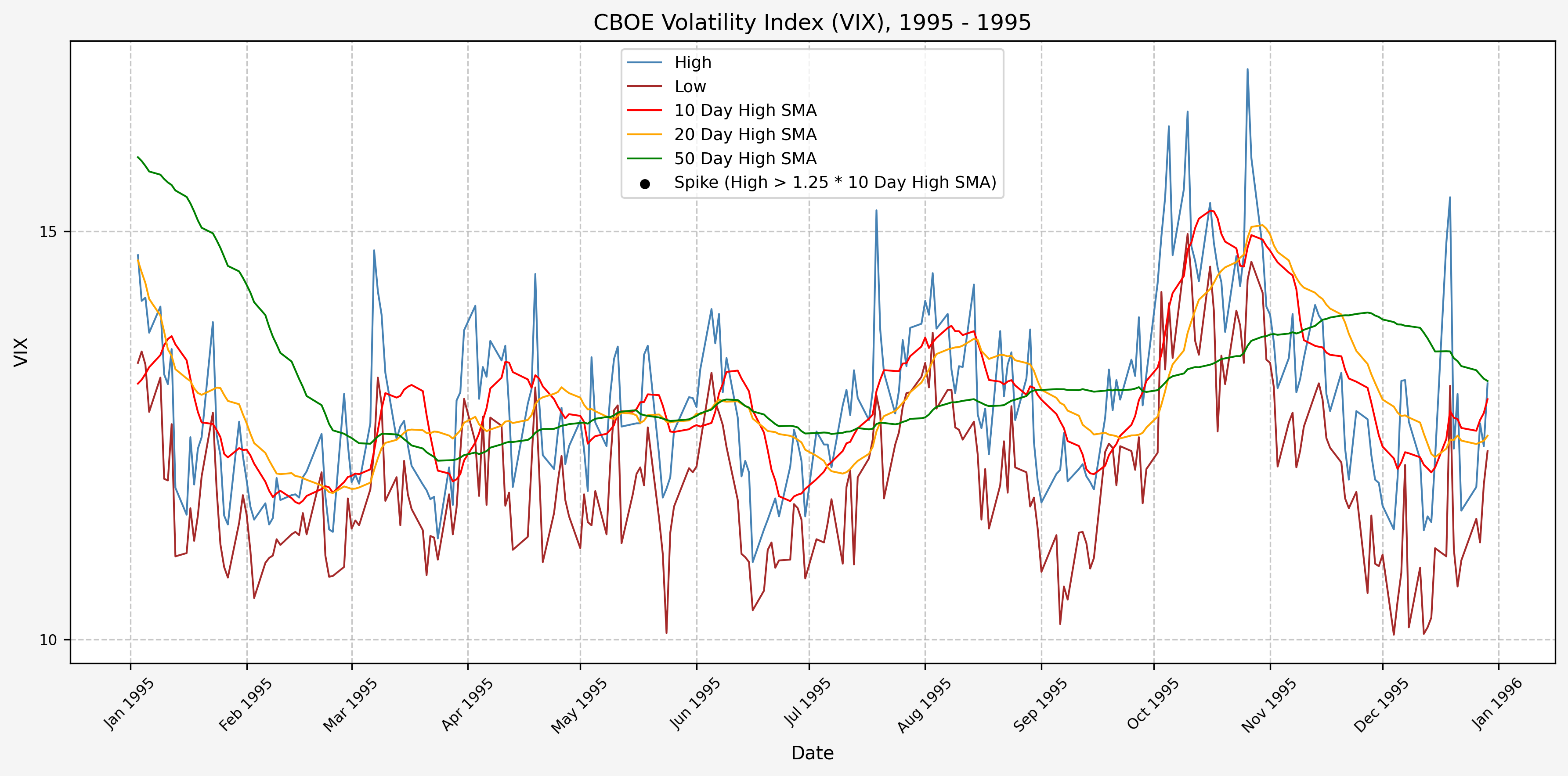
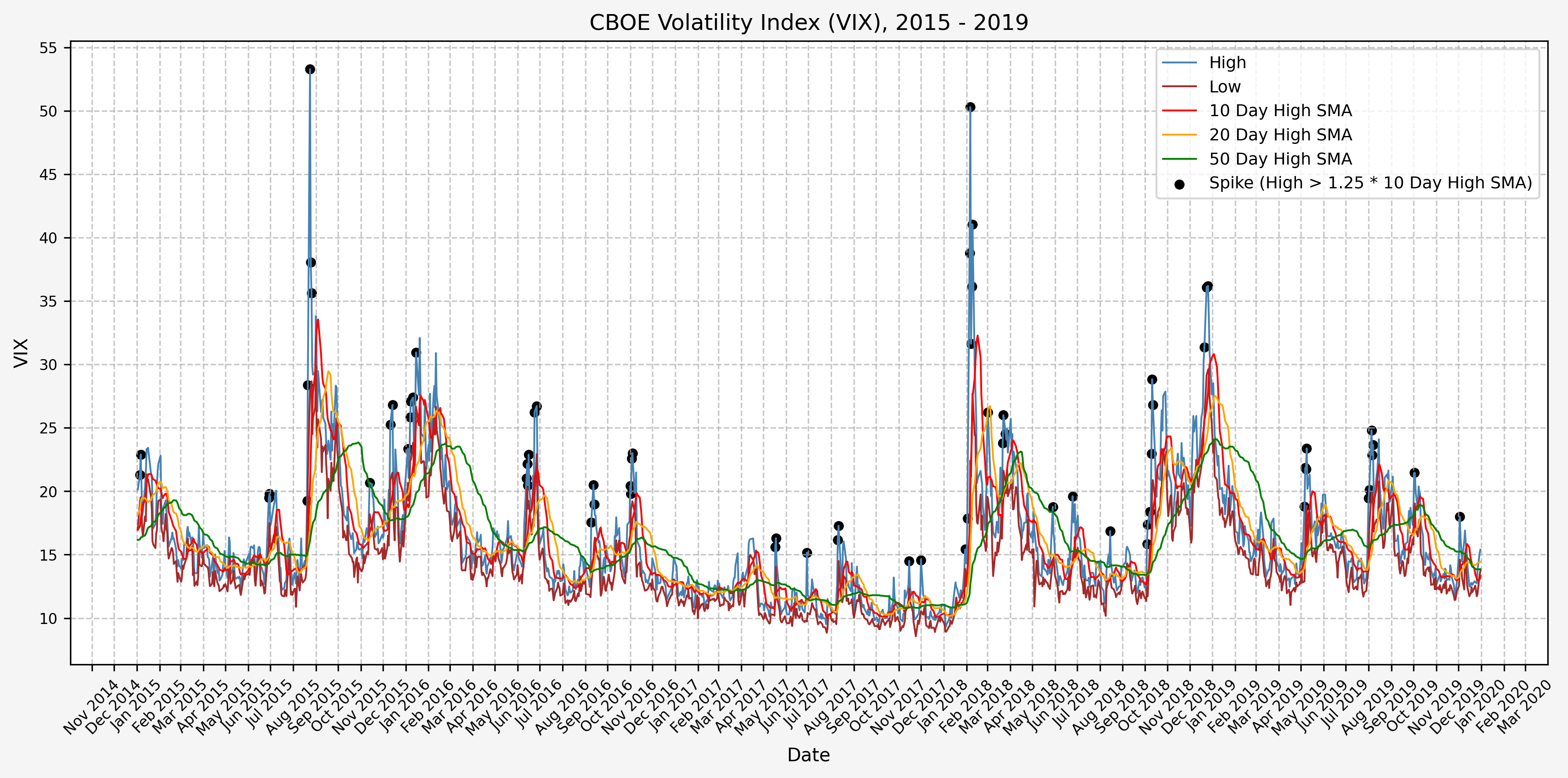
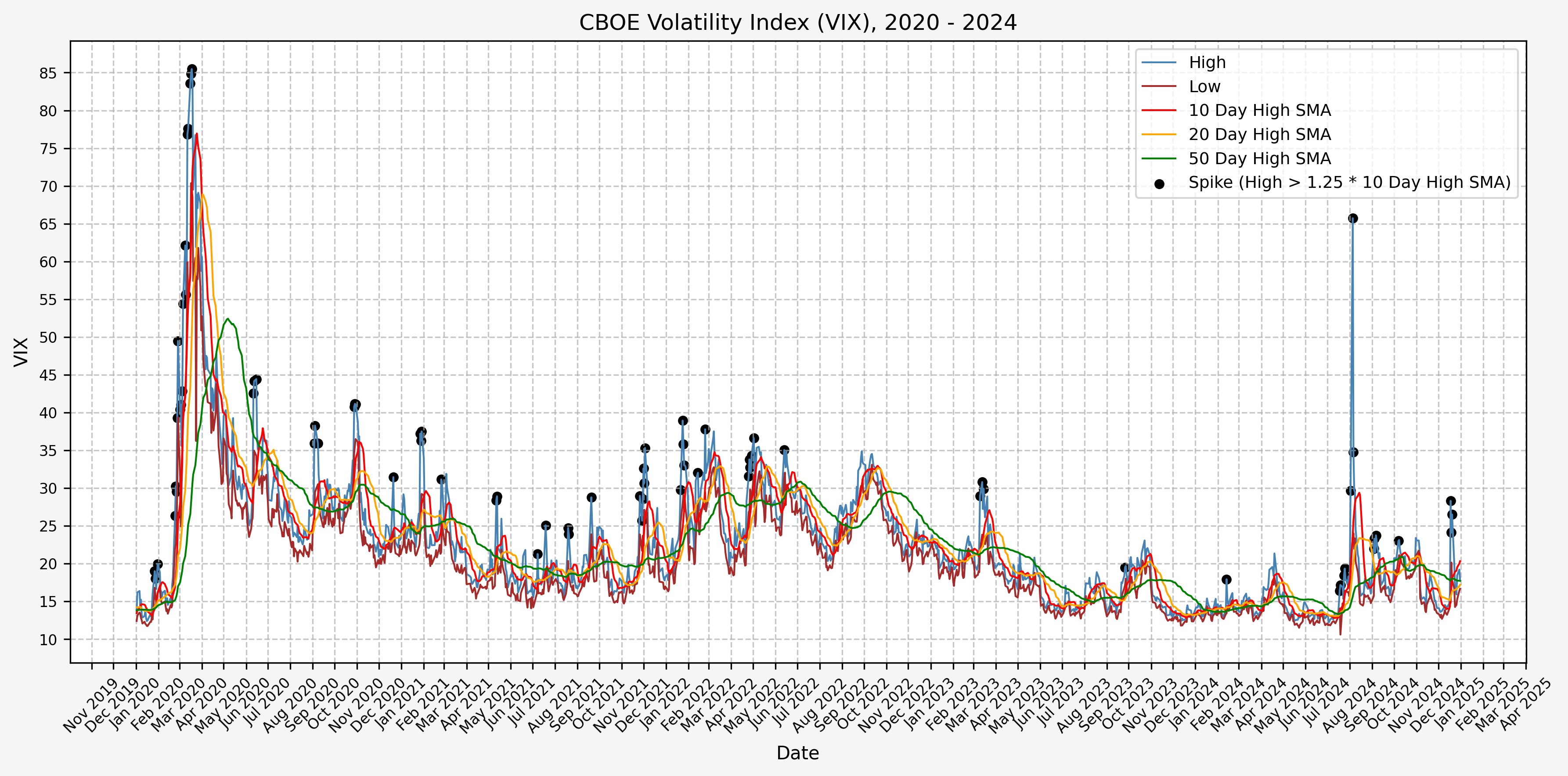
Next, we will consider the idea of a spike level in the VIX and how we might use a spike level to generate a signal. These elevated levels usually occur during market sell-off events or longer term drawdowns in the S&P 500. Sometimes the VIX reverts to recent levels after a spike, but other times levels remain elevated for weeks or even months.
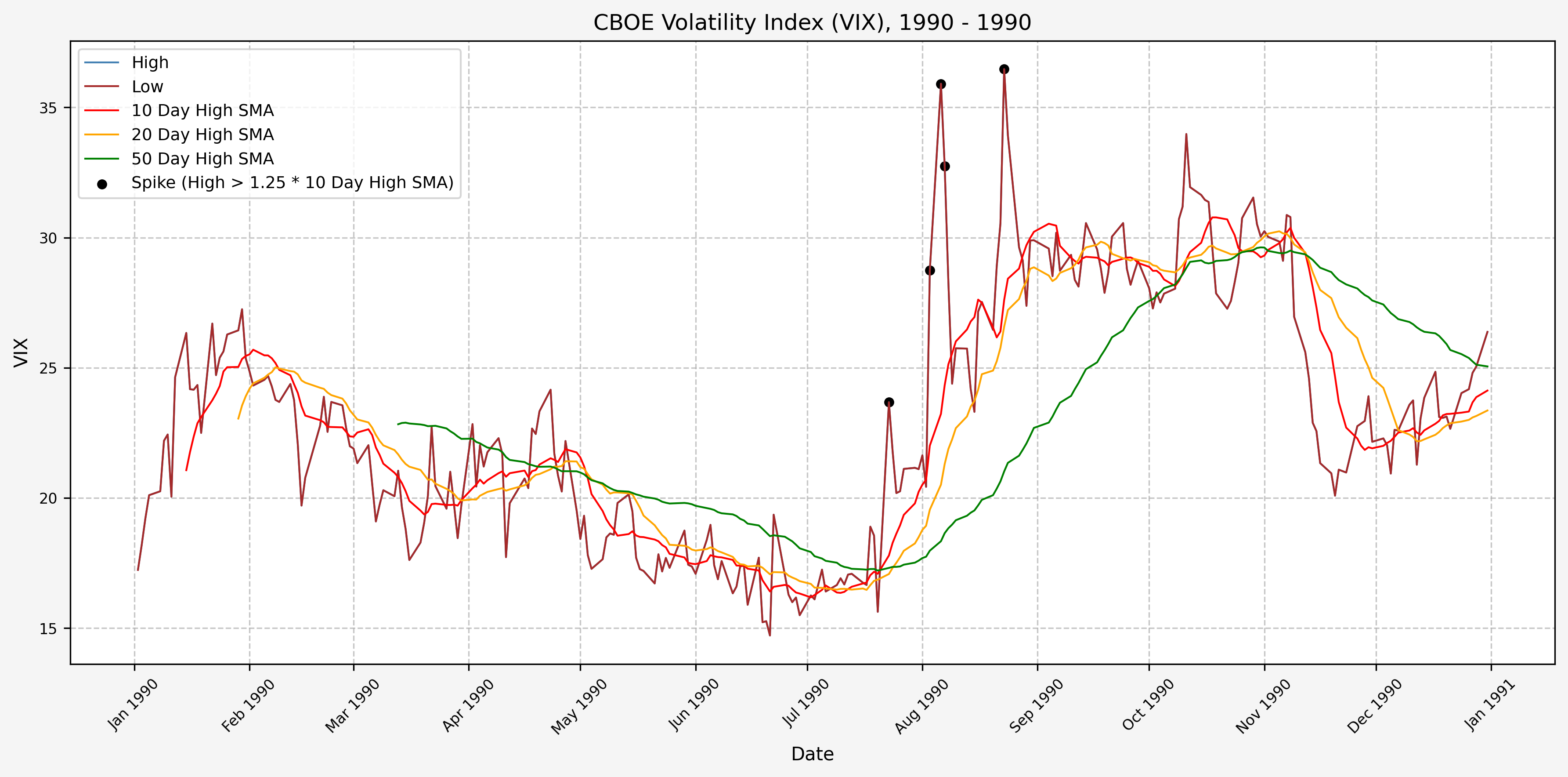
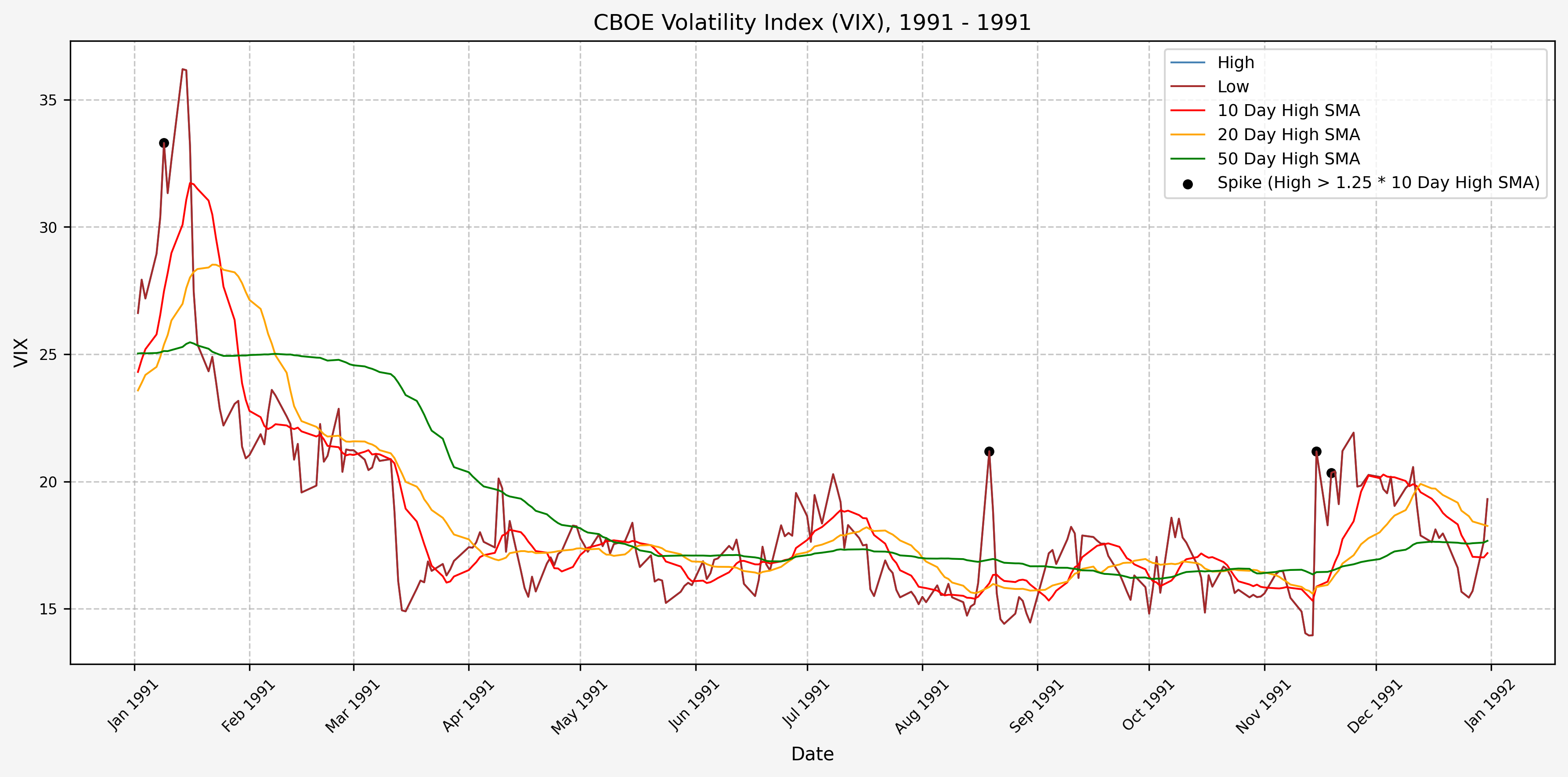
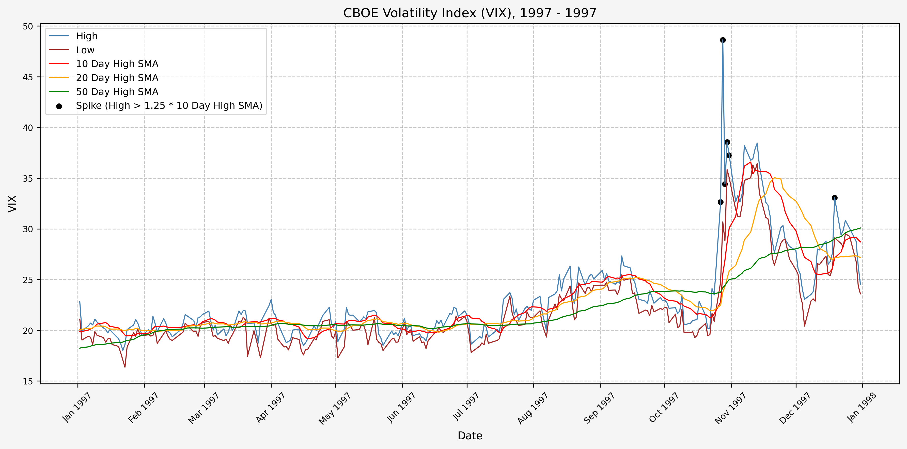
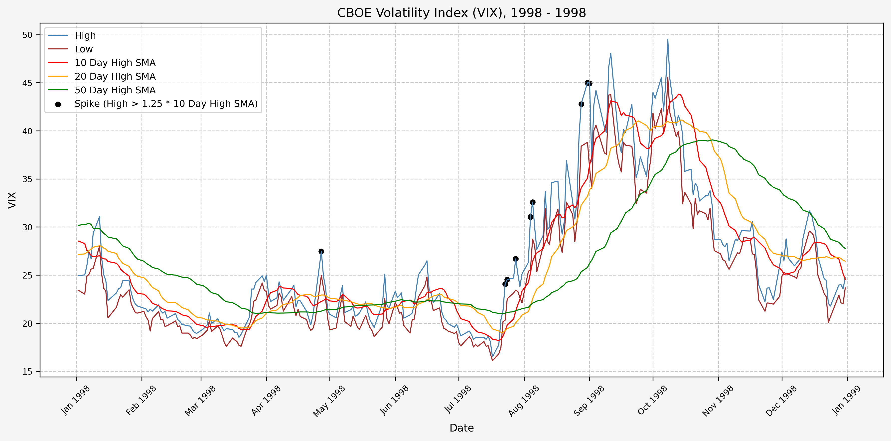
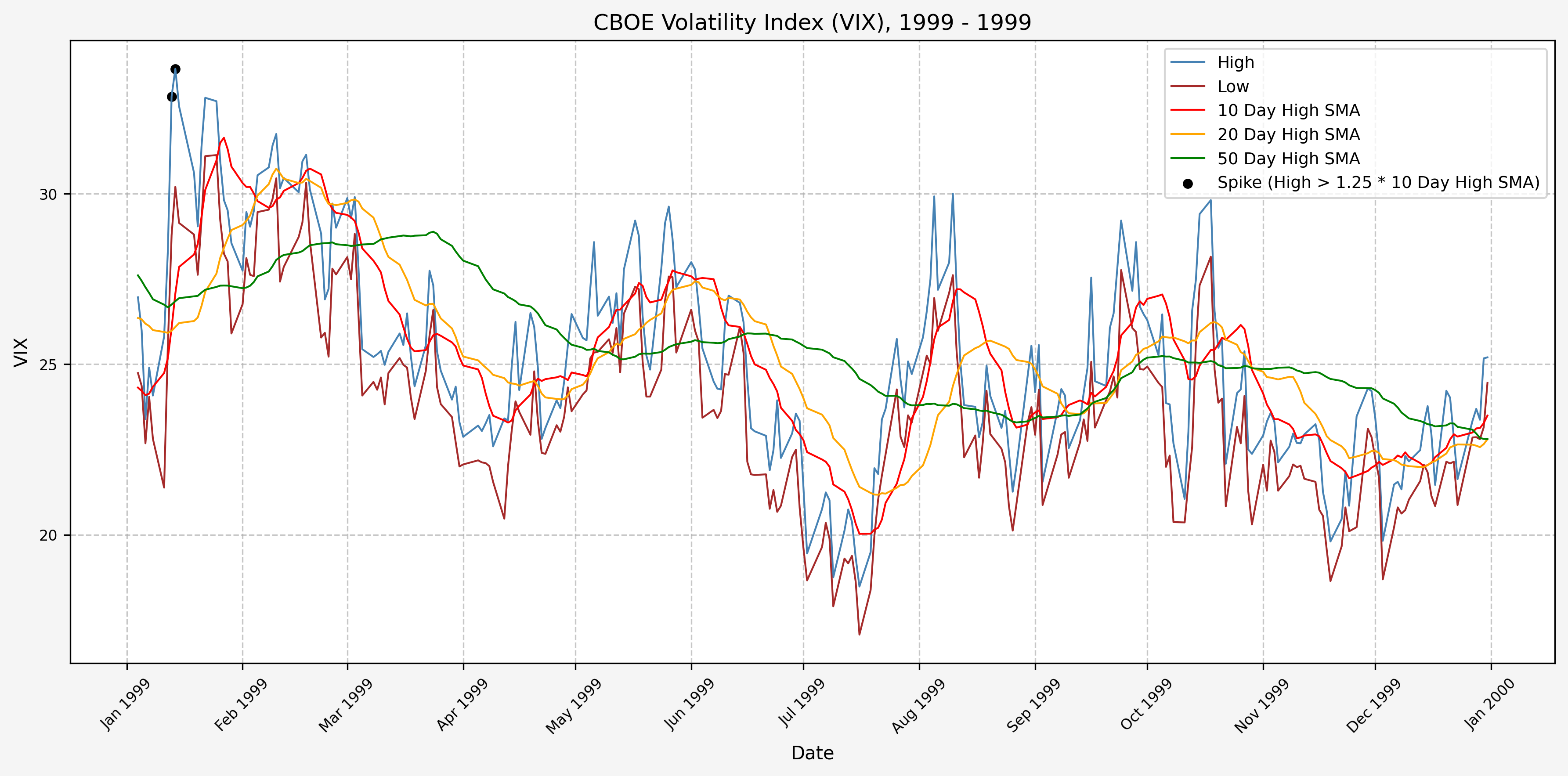
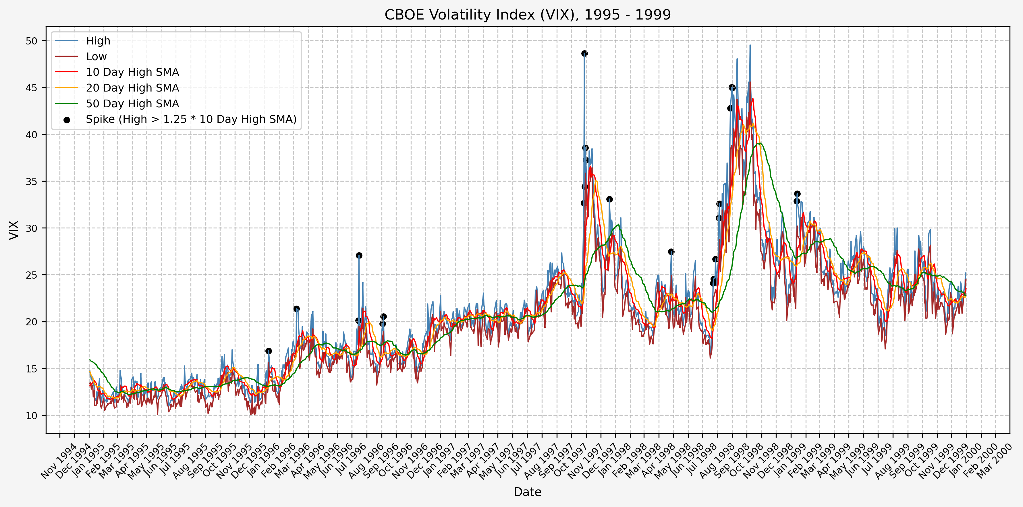
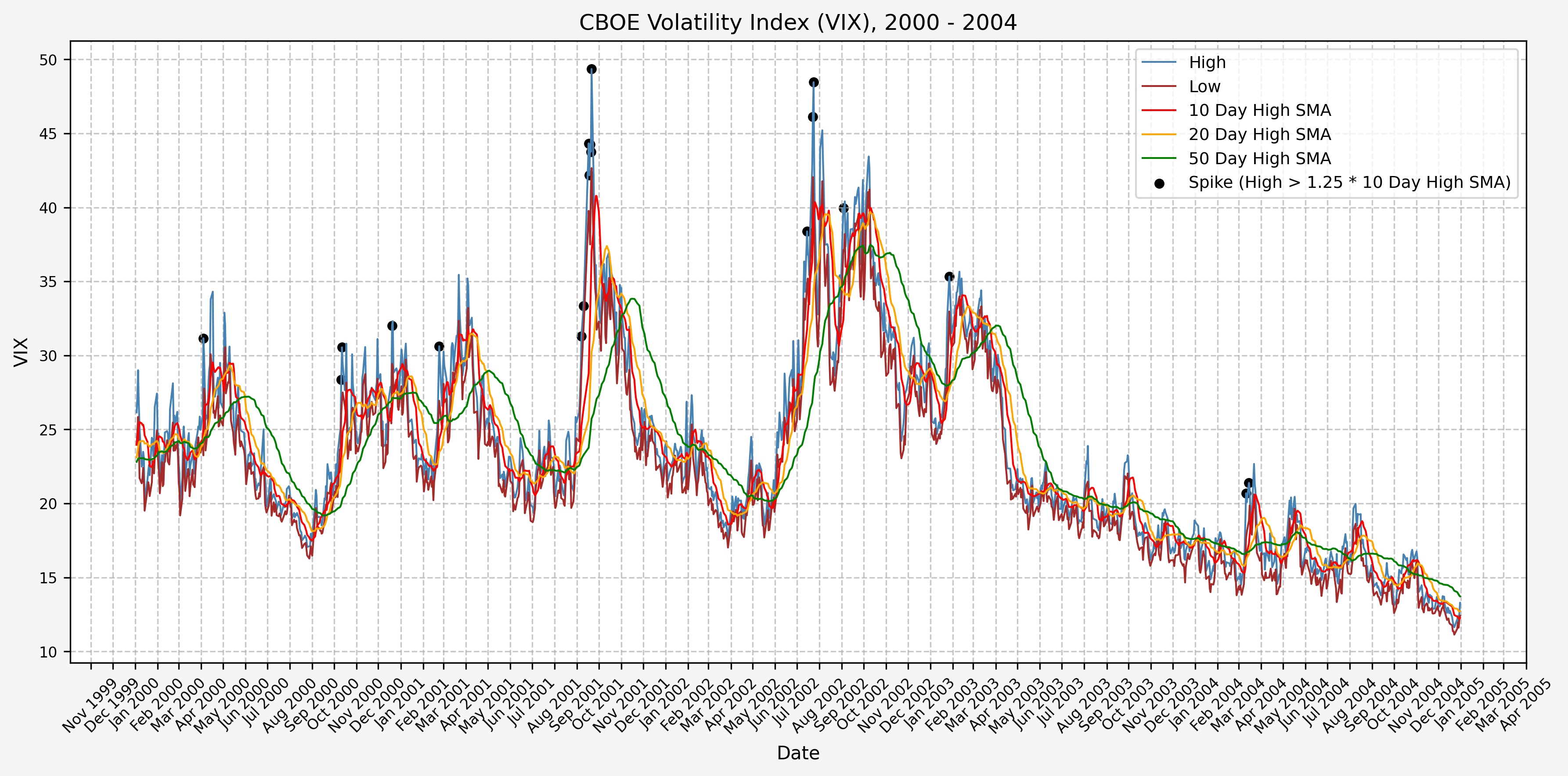
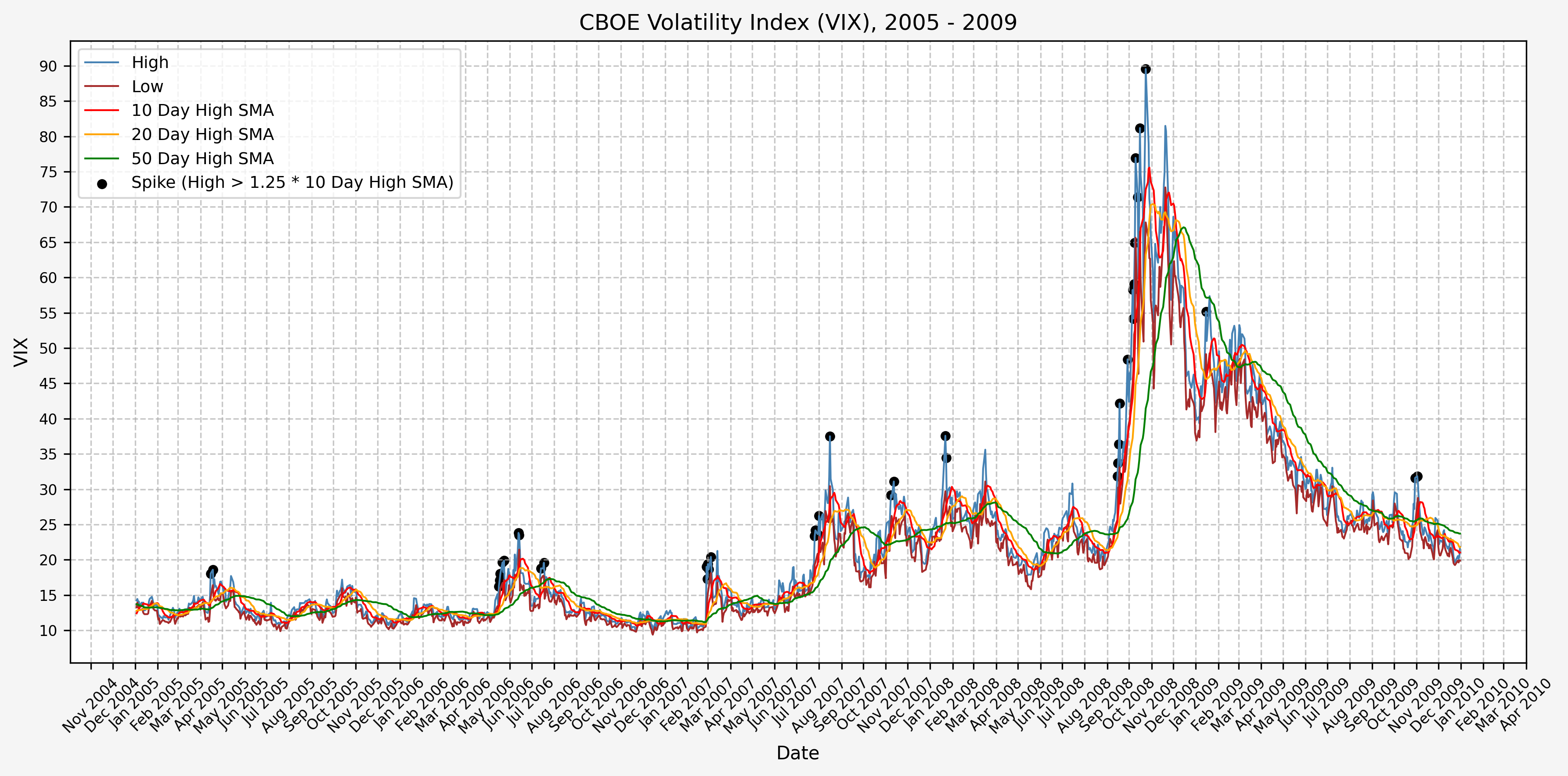
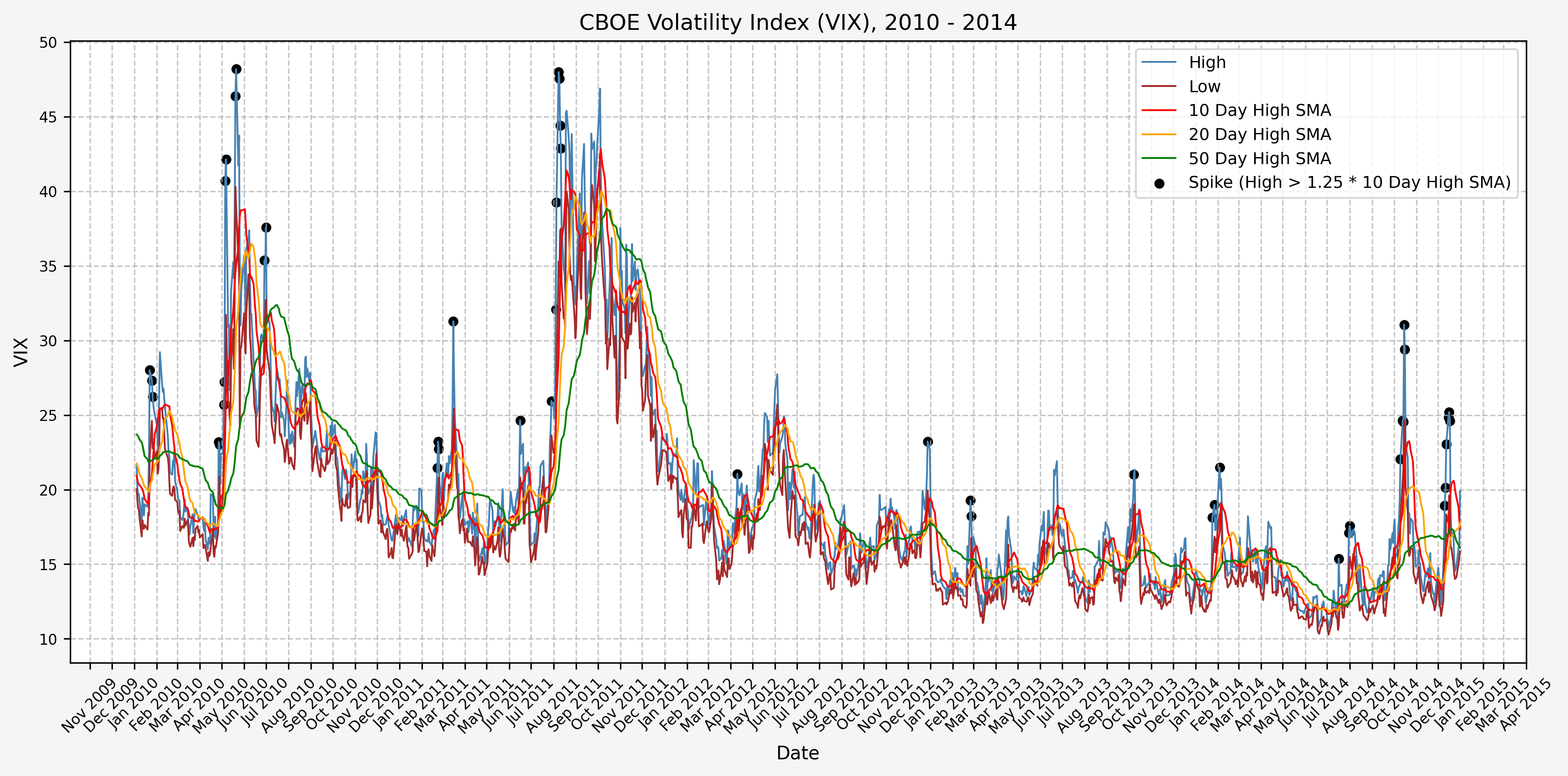
Determining A Spike Level
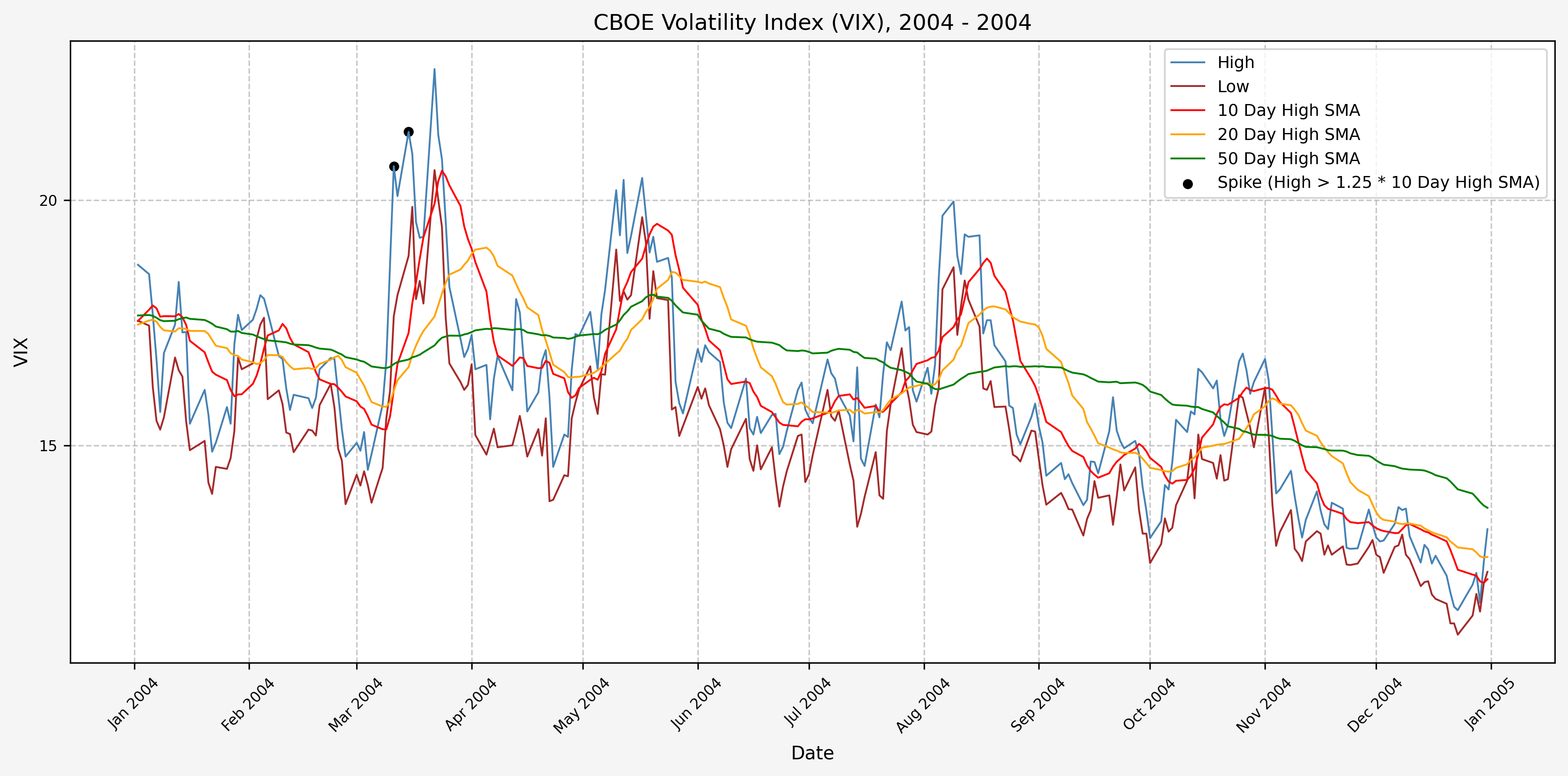
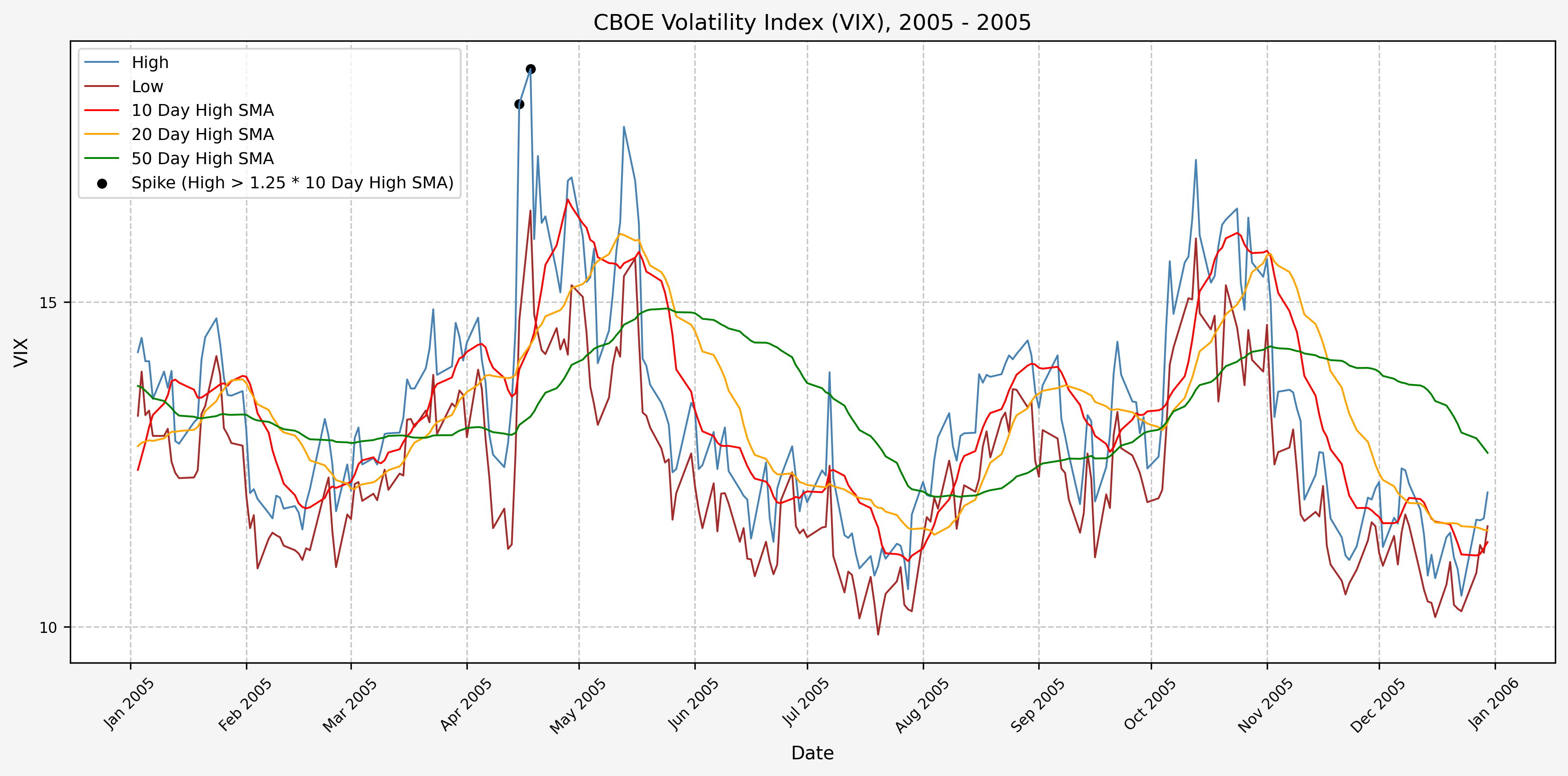
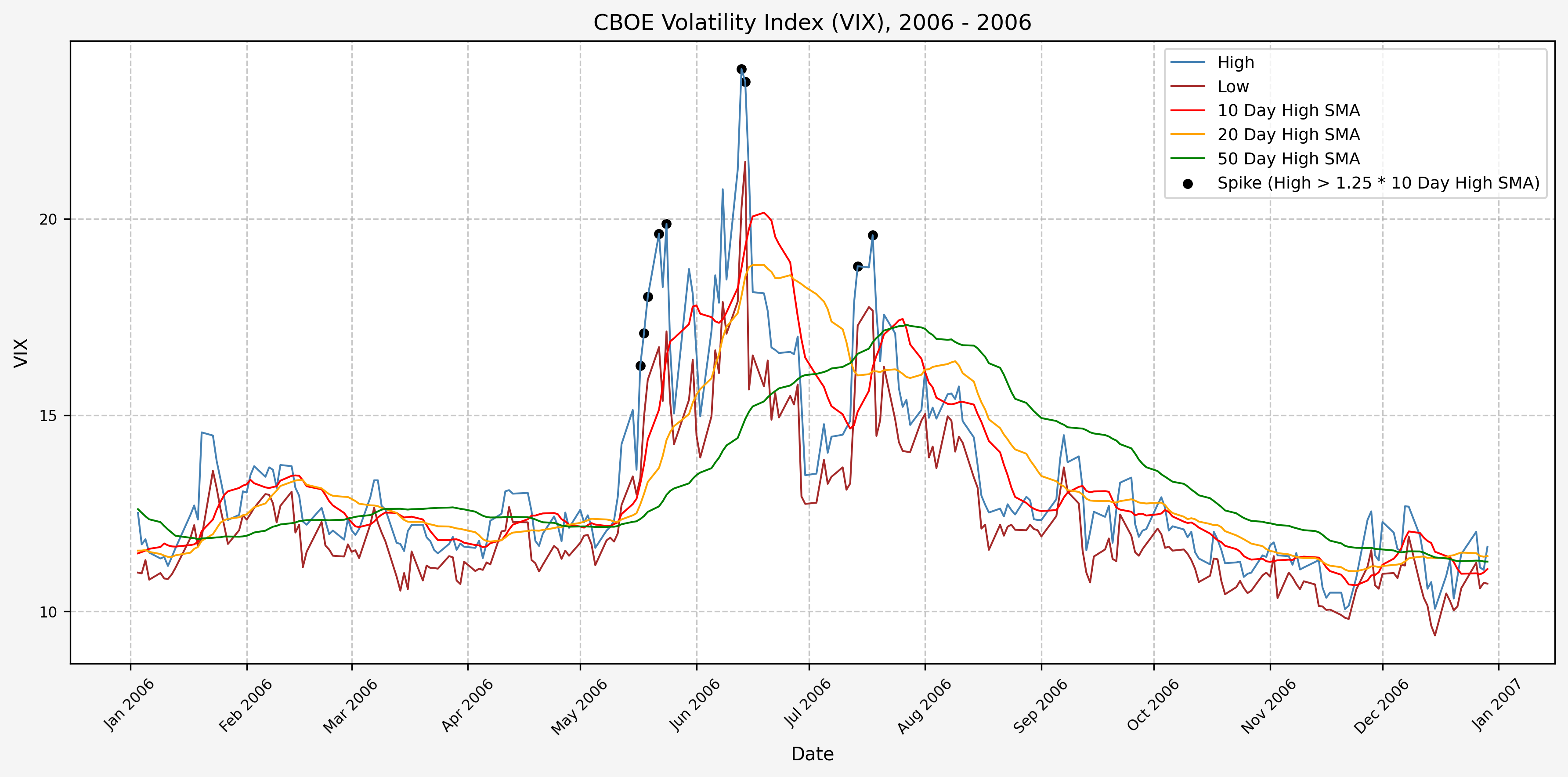
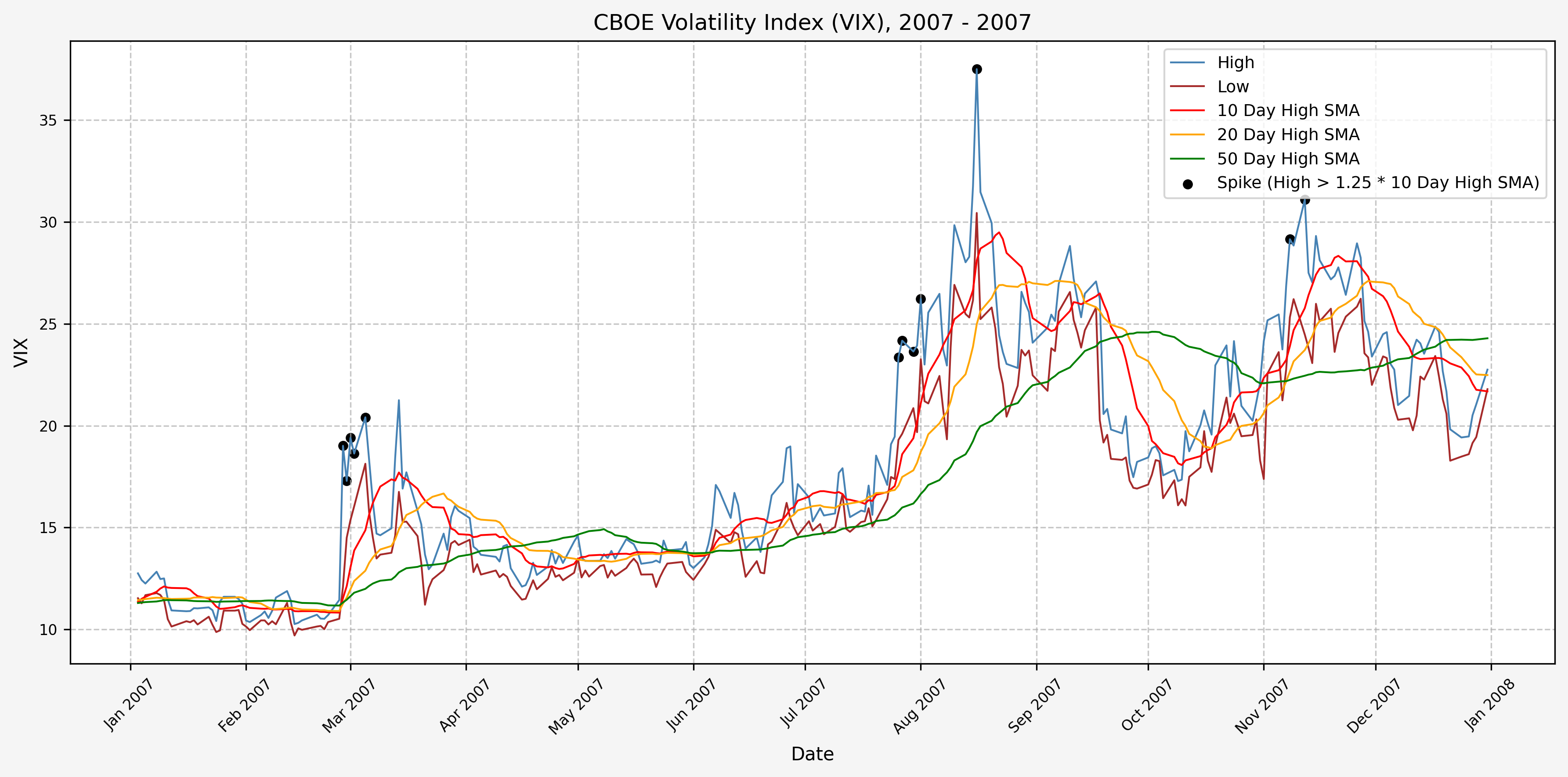
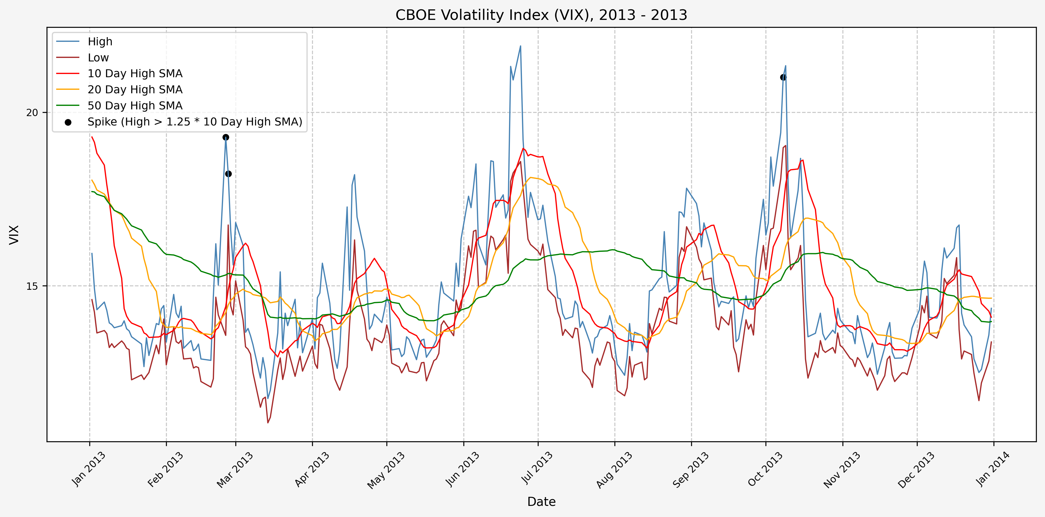
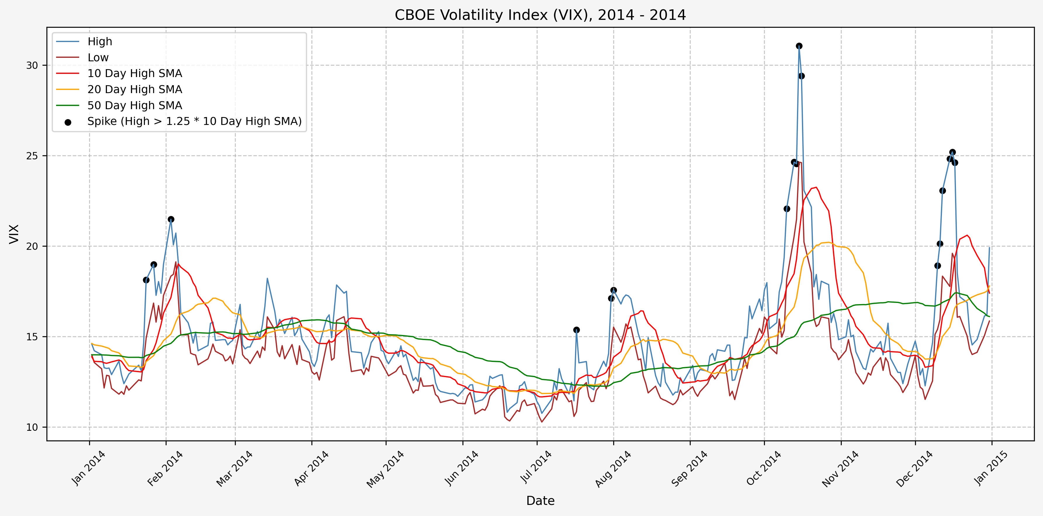
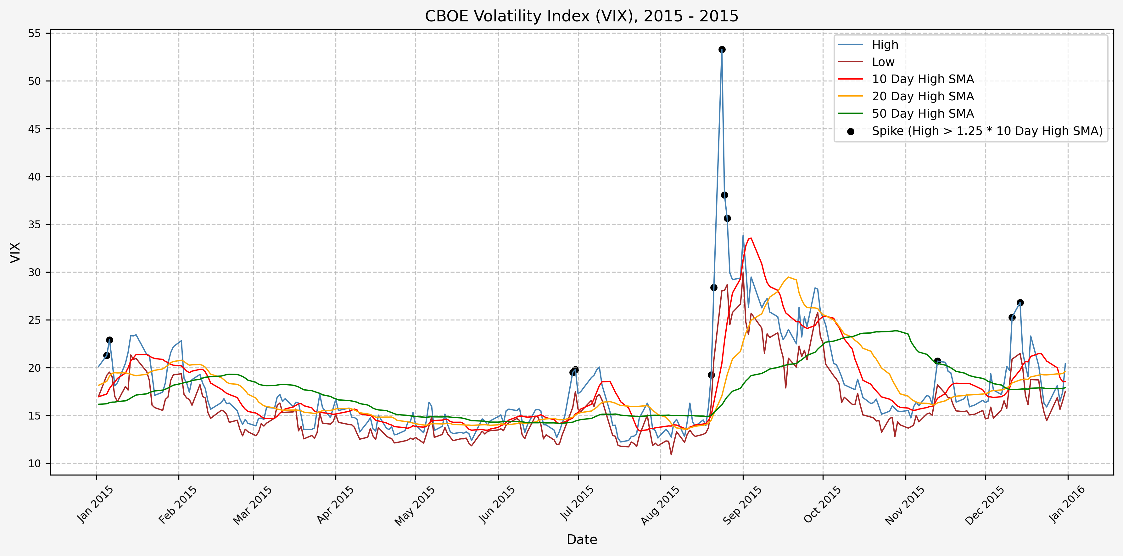
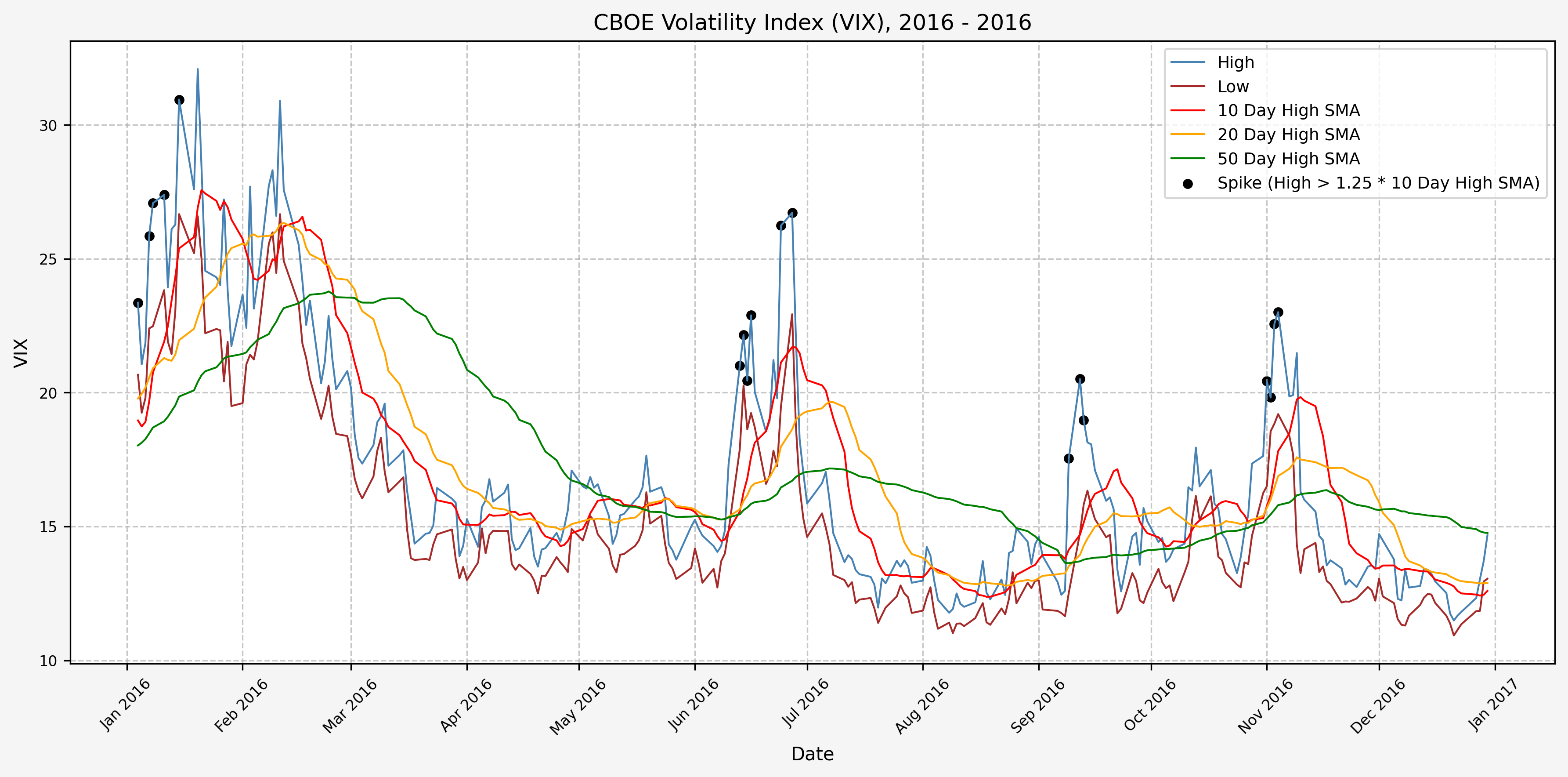
We will start the 10 day simple moving average (SMA) of the daily high level to get an idea of what is happening recently with the VIX. We’ll then pick an arbitrary spike level (25% above the 10 day SMA), and our signal is generated if the VIX hits a level that is above the spike threshold.
The idea is that the 10 day SMA will smooth out the recent short term volatility in the VIX, and therefore any gradual increases in the VIX are not interpreted as spike events.
We also will generate the 20 and 50 day SMAs for reference, and again to see what is happening with the level of the VIX over slightly longer timeframes.
Here’s the code for the above:
 1
 2
 3
 4
 5
 6
 7
 8
 9
10
11
12
13
14
15
16
17
18
19
20
21
22
23
24
25
26
27
28
29
30
31
32
33
34
35
36
37
38
39
40
41
42
43
44
45
46
| # Define the spike multiplier for detecting significant spikes
spike_level = 1.25
# =========================
# Simple Moving Averages (SMA)
# =========================
# Calculate 10-period SMA of 'High'
vix['High_SMA_10'] = vix['High'].rolling(window=10).mean()
# Shift the 10-period SMA by 1 to compare with current 'High'
vix['High_SMA_10_Shift'] = vix['High_SMA_10'].shift(1)
# Calculate the spike level based on shifted SMA and spike multiplier
vix['Spike_Level_SMA'] = vix['High_SMA_10_Shift'] * spike_level
# Calculate 20-period SMA of 'High'
vix['High_SMA_20'] = vix['High'].rolling(window=20).mean()
# Determine if 'High' exceeds the spike level (indicates a spike)
vix['Spike_SMA'] = vix['High'] >= vix['Spike_Level_SMA']
# Calculate 50-period SMA of 'High' for trend analysis
vix['High_SMA_50'] = vix['High'].rolling(window=50).mean()
# =========================
# Exponential Moving Averages (EMA)
# =========================
# Calculate 10-period EMA of 'High'
vix['High_EMA_10'] = vix['High'].ewm(span=10, adjust=False).mean()
# Shift the 10-period EMA by 1 to compare with current 'High'
vix['High_EMA_10_Shift'] = vix['High_EMA_10'].shift(1)
# Calculate the spike level based on shifted EMA and spike multiplier
vix['Spike_Level_EMA'] = vix['High_EMA_10_Shift'] * spike_level
# Calculate 20-period EMA of 'High'
vix['High_EMA_20'] = vix['High'].ewm(span=20, adjust=False).mean()
# Determine if 'High' exceeds the spike level (indicates a spike)
vix['Spike_EMA'] = vix['High'] >= vix['Spike_Level_EMA']
# Calculate 50-period EMA of 'High' for trend analysis
vix['High_EMA_50'] = vix['High'].ewm(span=50, adjust=False).mean()
|
For this exercise, we will use simple moving averages.
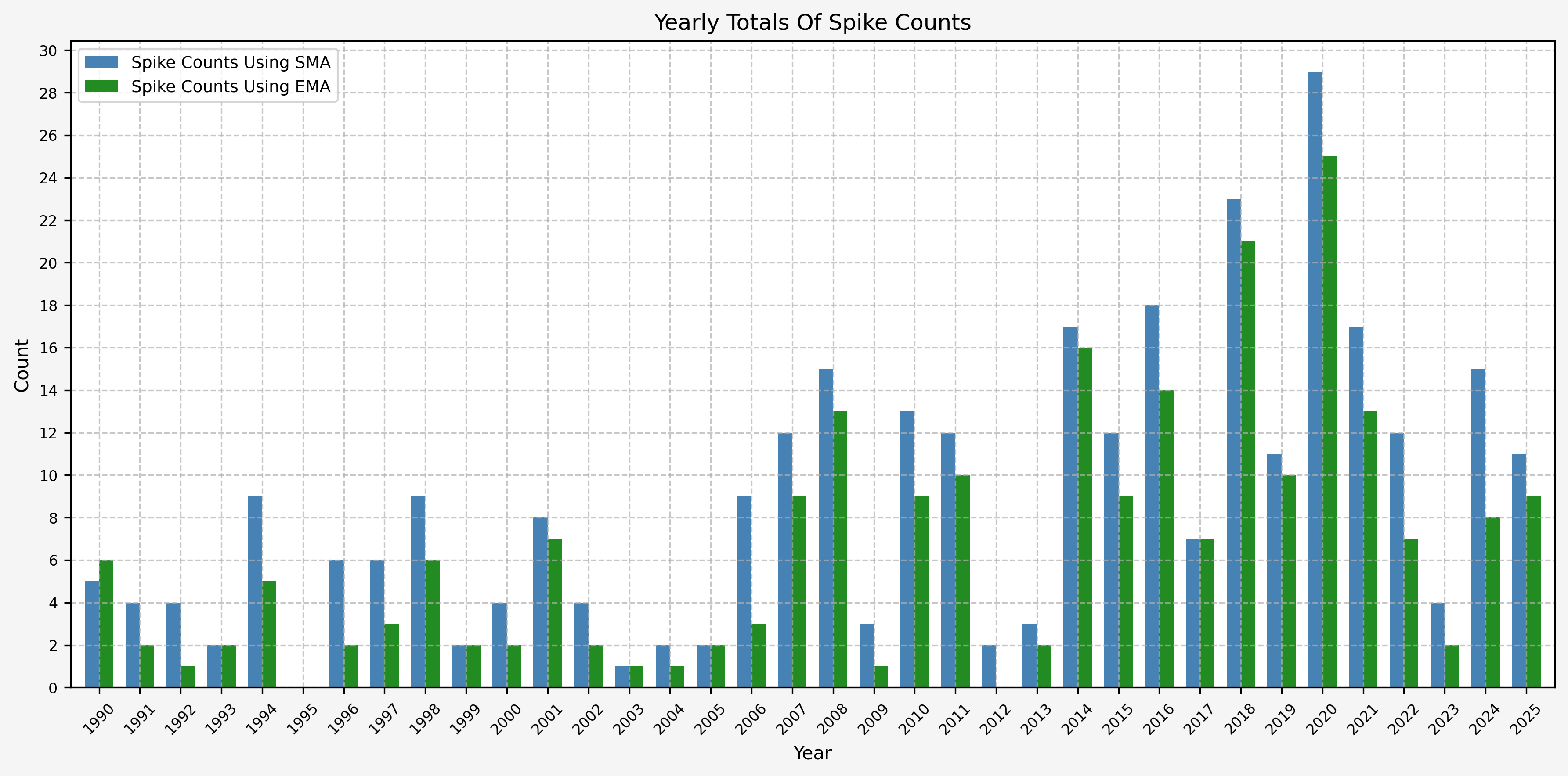
Spike Counts (Signals) By Year
To investigate the number of spike events (or signals) that we receive on a yearly basis, we can run the following:
 1
 2
 3
 4
 5
 6
 7
 8
 9
10
| # Ensure the index is a DatetimeIndex
vix.index = pd.to_datetime(vix.index)
# Create a new column for the year extracted from the date index
vix['Year'] = vix.index.year
# Group by year and the "Spike_SMA" and "Spike_EMA" columns, then count occurrences
spike_count_SMA = vix.groupby(['Year', 'Spike_SMA']).size().unstack(fill_value=0)
spike_count_SMA
|
Which gives us the following:
| Year | False | True |
|---|
| 1990 | 248 | 5 |
| 1991 | 249 | 4 |
| 1992 | 250 | 4 |
| 1993 | 251 | 2 |
| 1994 | 243 | 9 |
| 1995 | 252 | 0 |
| 1996 | 248 | 6 |
| 1997 | 247 | 6 |
| 1998 | 243 | 9 |
| 1999 | 250 | 2 |
| 2000 | 248 | 4 |
| 2001 | 240 | 8 |
| 2002 | 248 | 4 |
| 2003 | 251 | 1 |
| 2004 | 250 | 2 |
| 2005 | 250 | 2 |
| 2006 | 242 | 9 |
| 2007 | 239 | 12 |
| 2008 | 238 | 15 |
| 2009 | 249 | 3 |
| 2010 | 239 | 13 |
| 2011 | 240 | 12 |
| 2012 | 248 | 2 |
| 2013 | 249 | 3 |
| 2014 | 235 | 17 |
| 2015 | 240 | 12 |
| 2016 | 234 | 18 |
| 2017 | 244 | 7 |
| 2018 | 228 | 23 |
| 2019 | 241 | 11 |
| 2020 | 224 | 29 |
| 2021 | 235 | 17 |
| 2022 | 239 | 12 |
| 2023 | 246 | 4 |
| 2024 | 237 | 15 |
| 2025 | 67 | 11 |
And the plot to aid with visualization. Based on the plot, it seems as though volatility has increased since the early 2000’s:
Spike Counts (Signals) Plots By Year
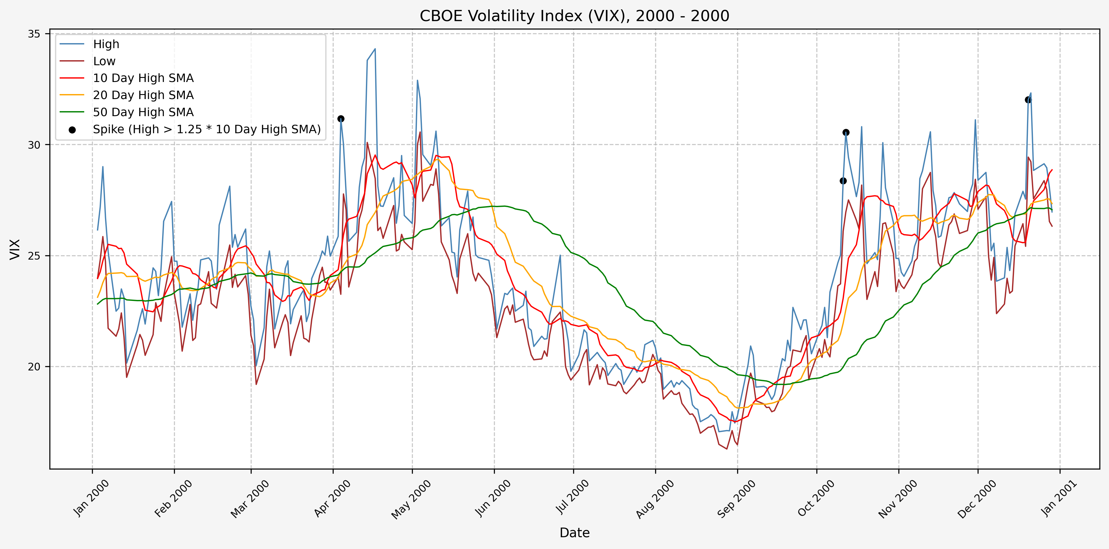
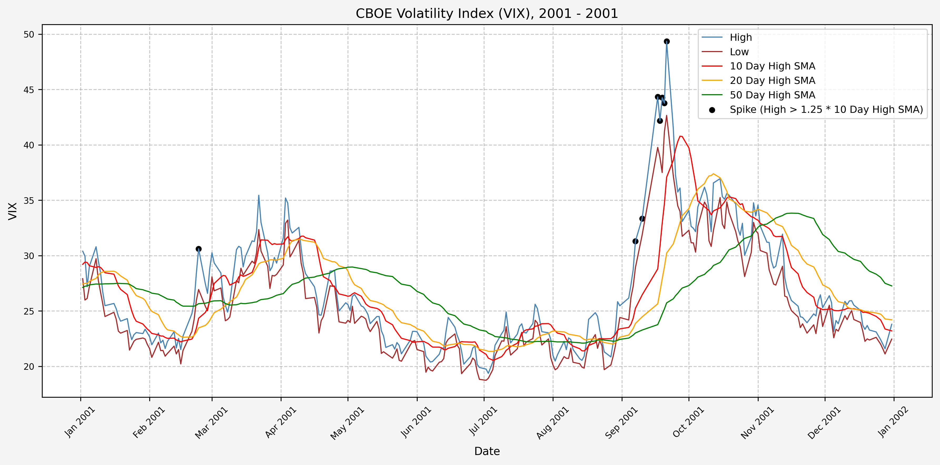
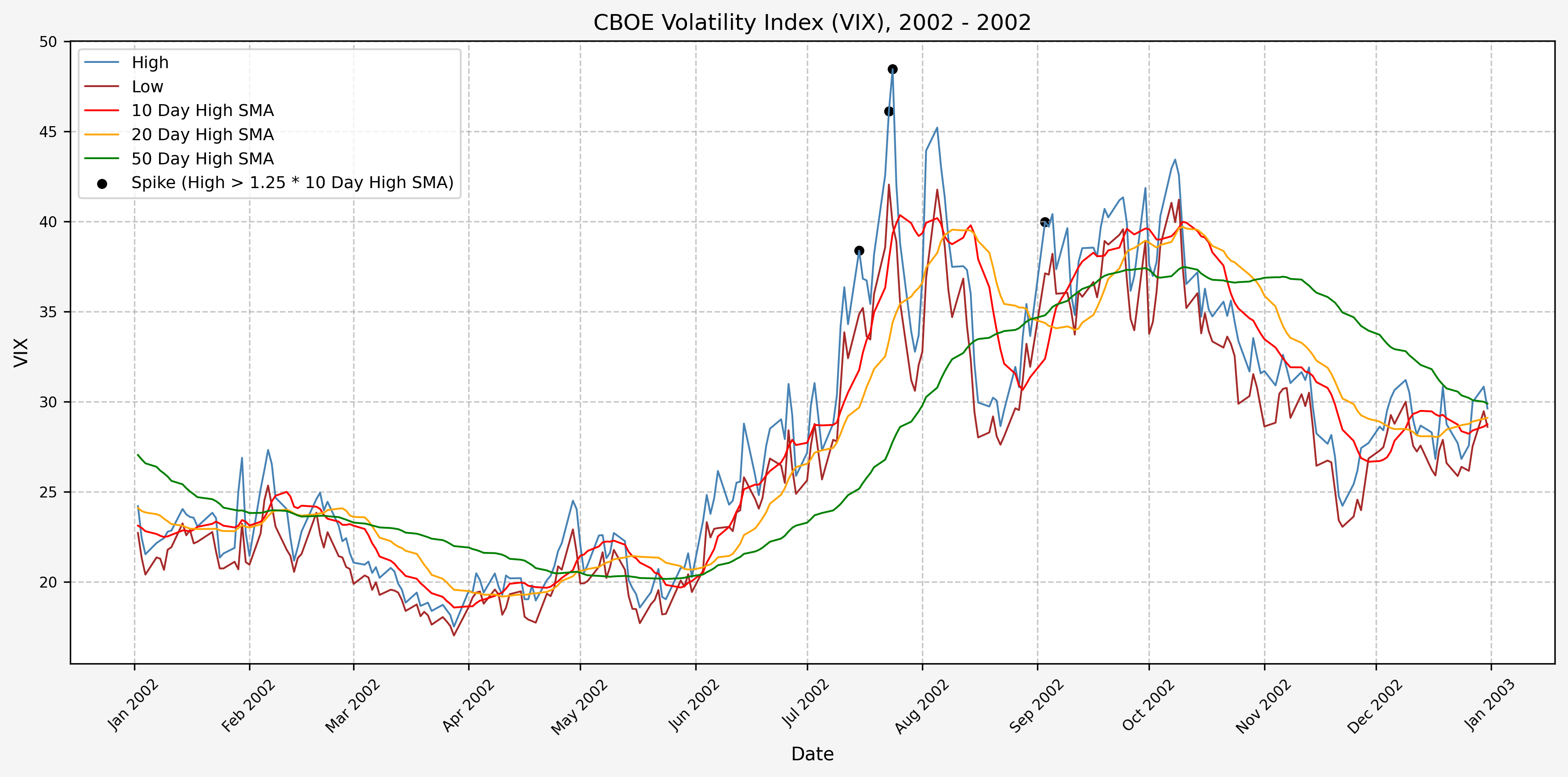
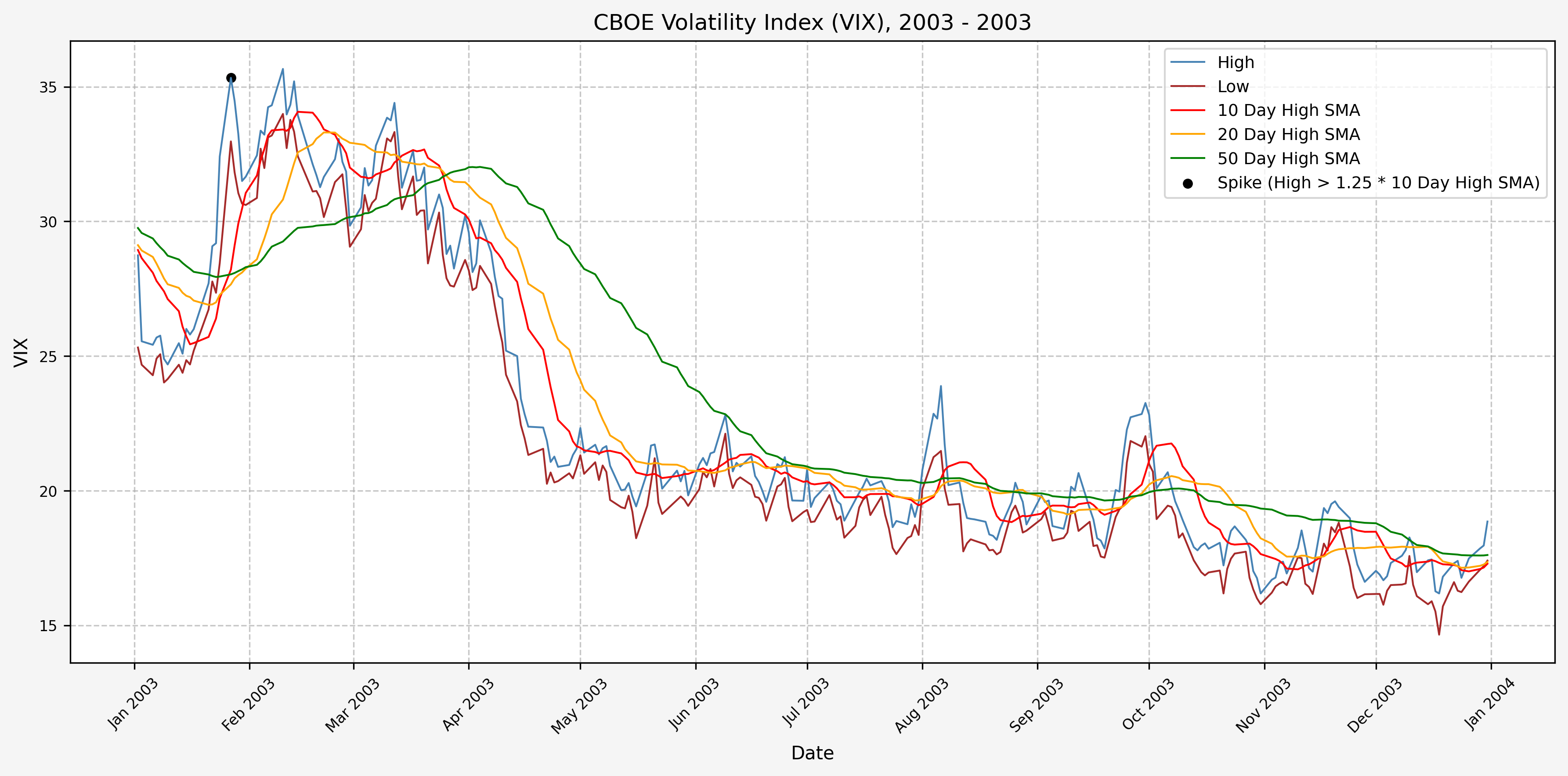
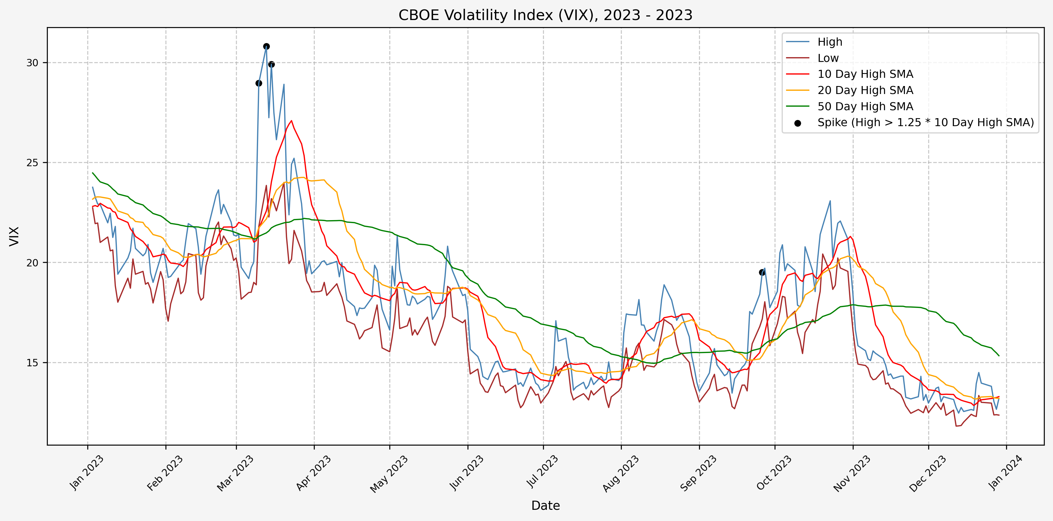
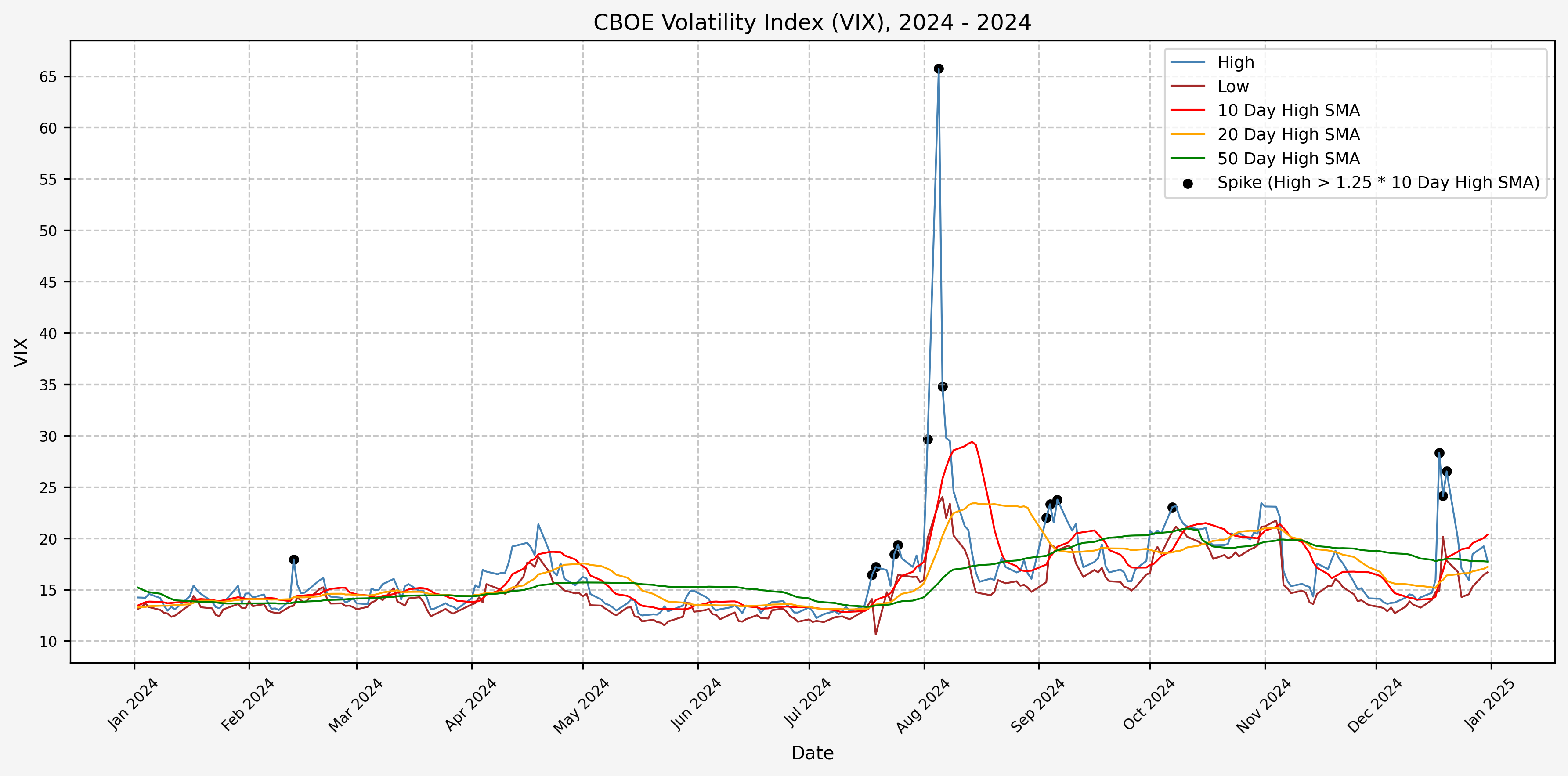
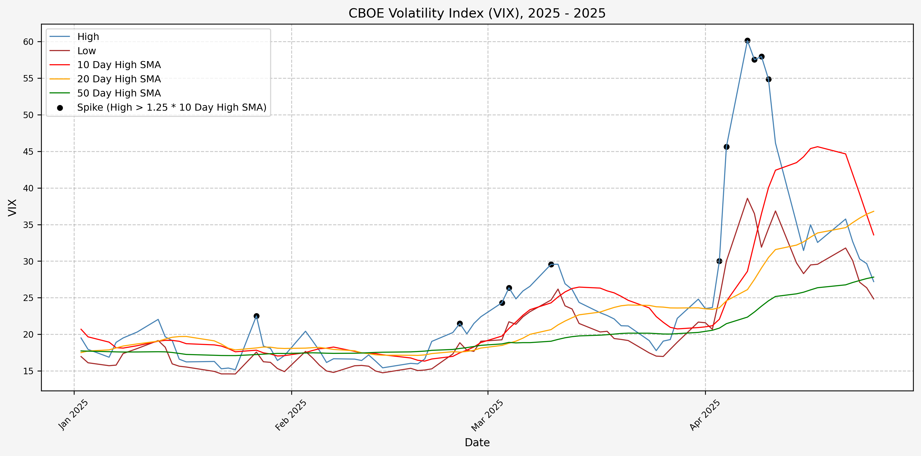
Here are the yearly plots for when signals are generated:
1990
1991
1992
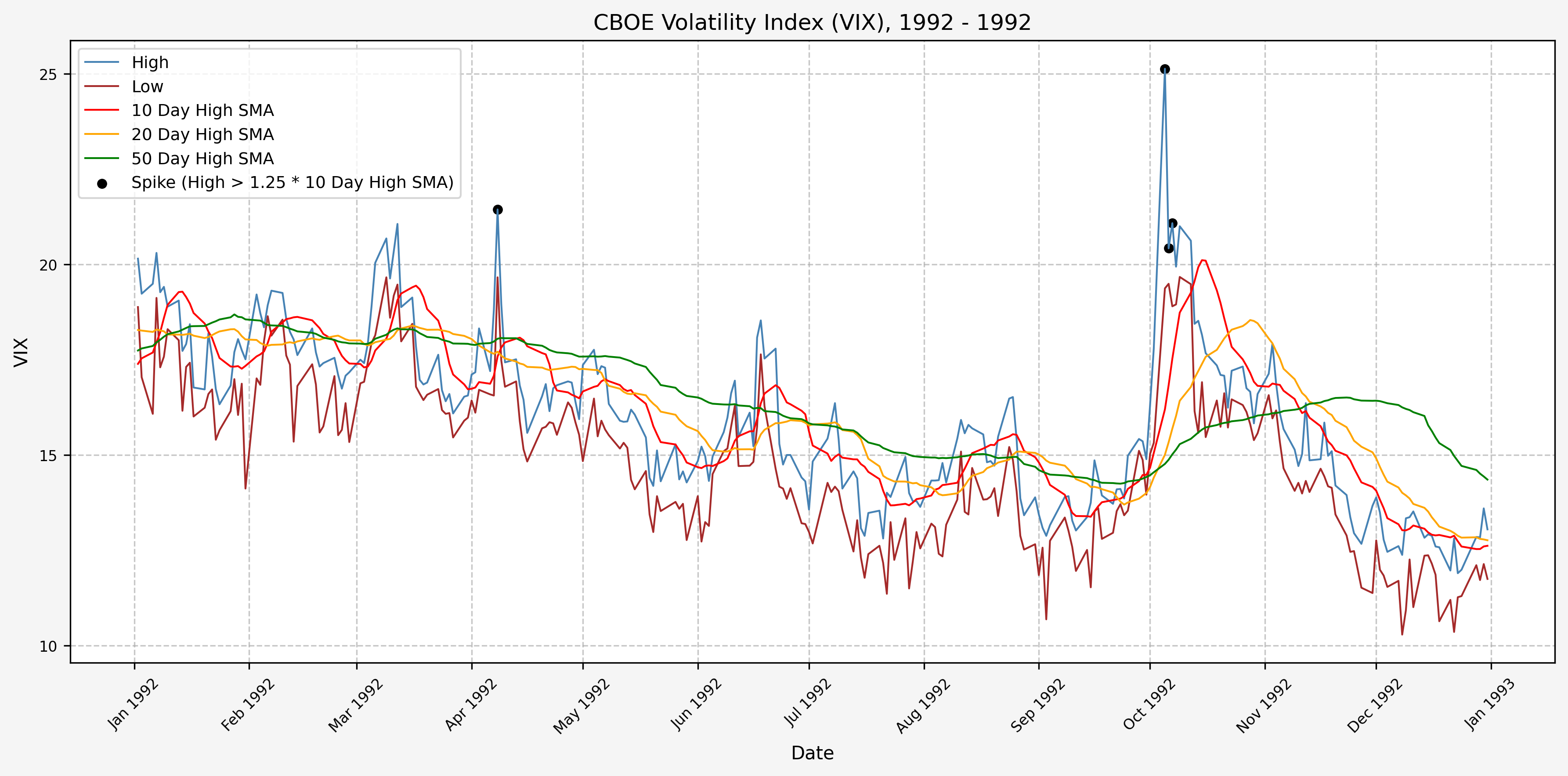
1993
1994
1995
1996
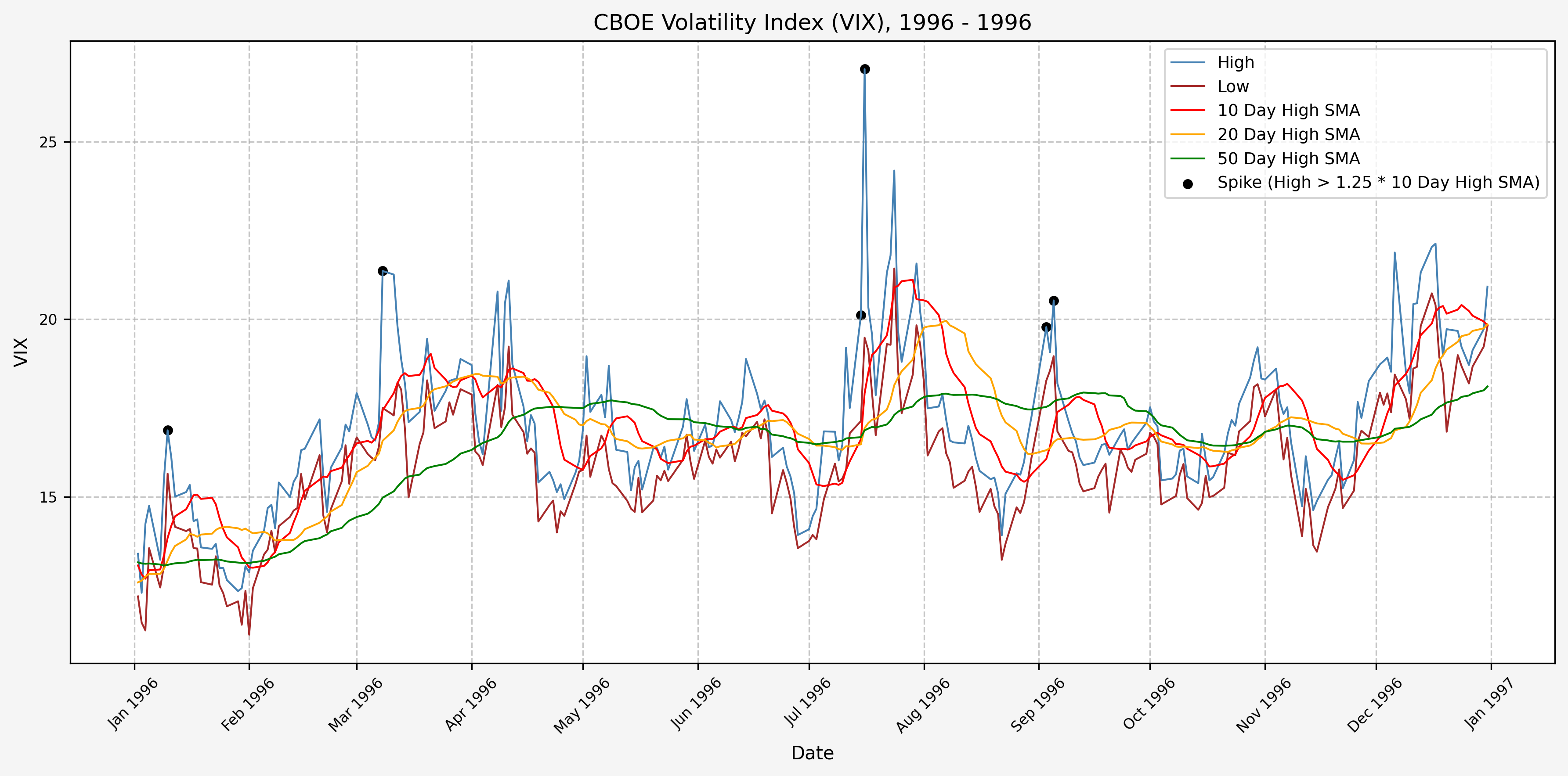
1997
1998
1999
2000
2001
2002
2003
2004
2005
2006
2007
2008
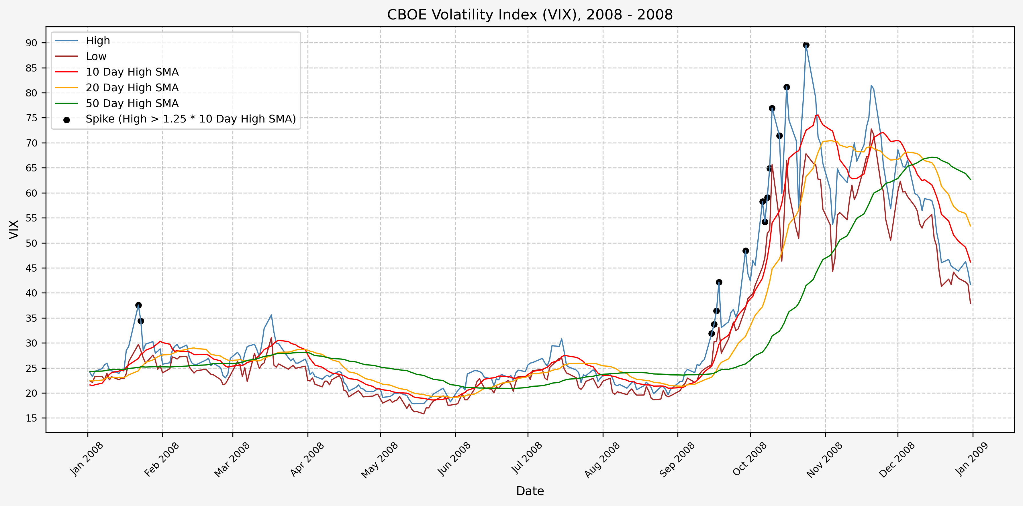
2009

2010
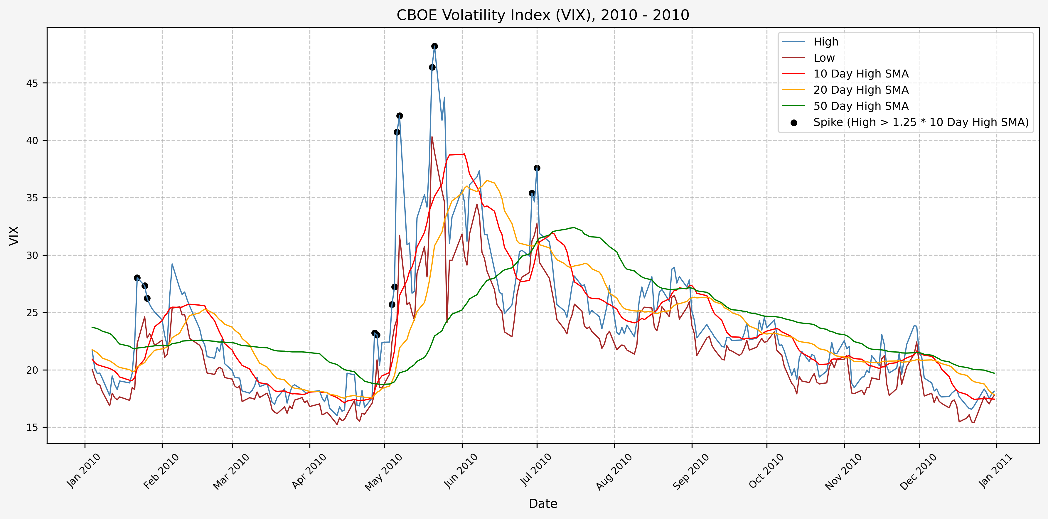
2011
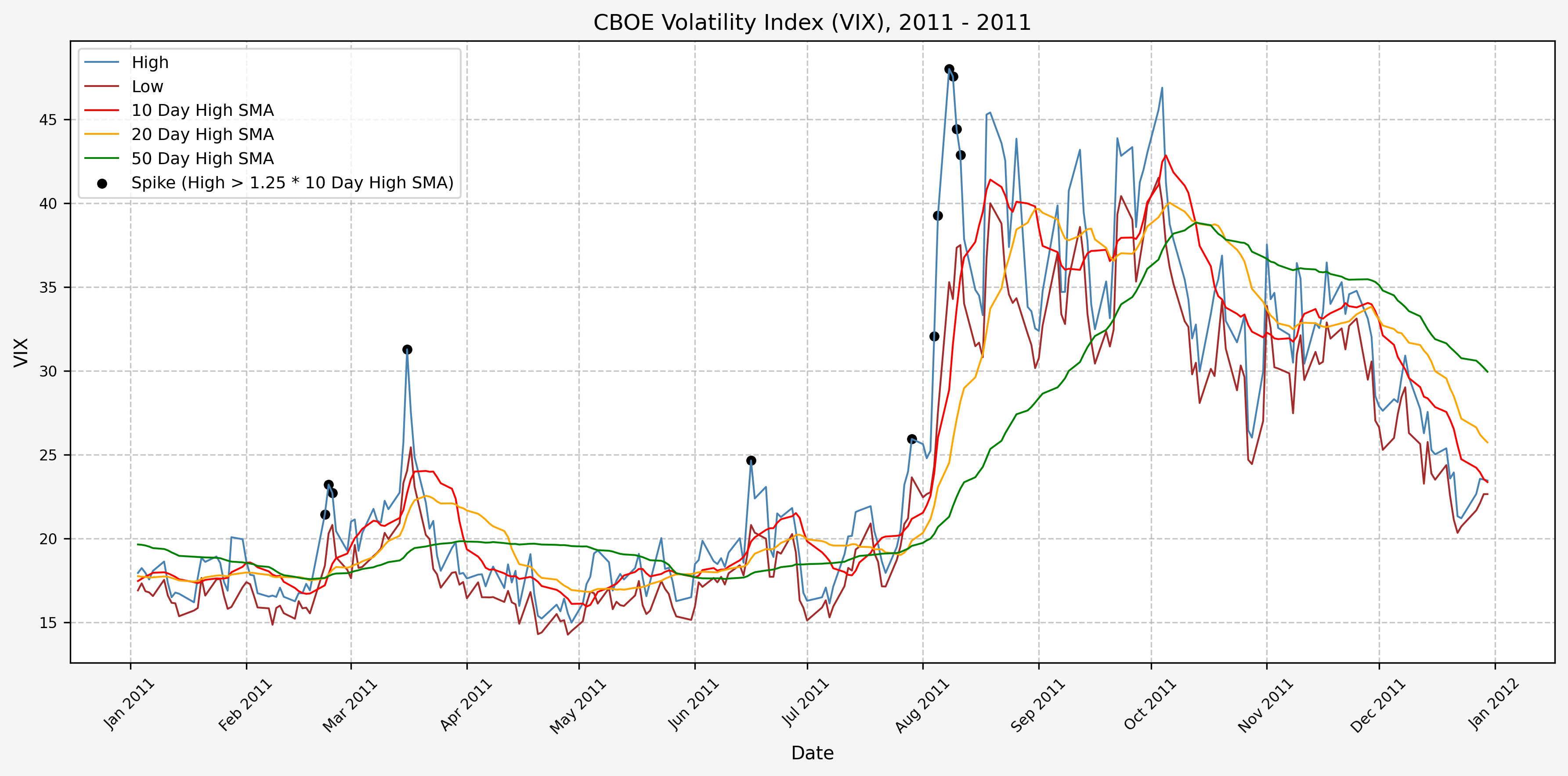
2012
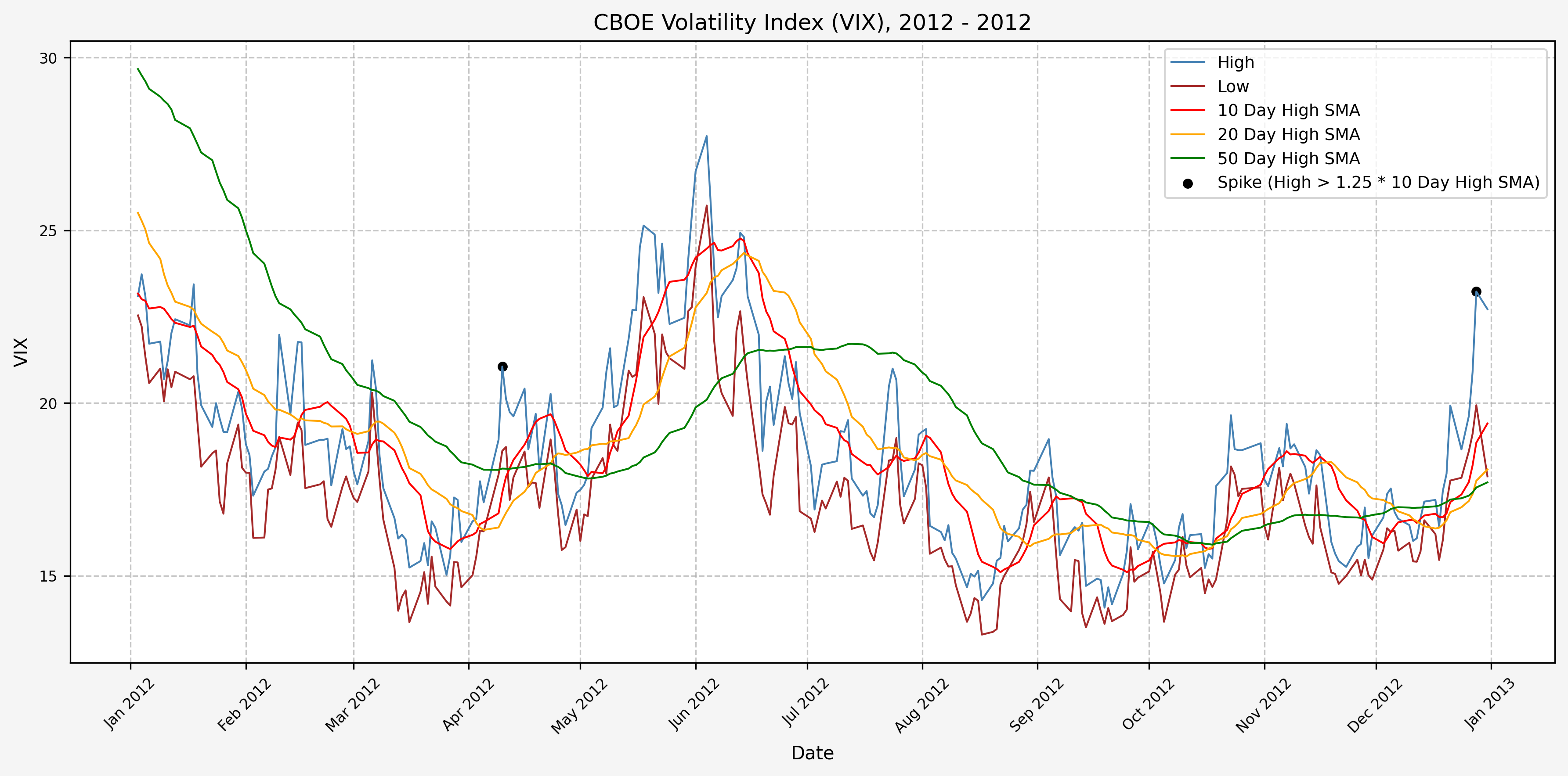
2013
2014
2015
2016
2017
2018
2019

2020
2021
2022

2023
2024
2025
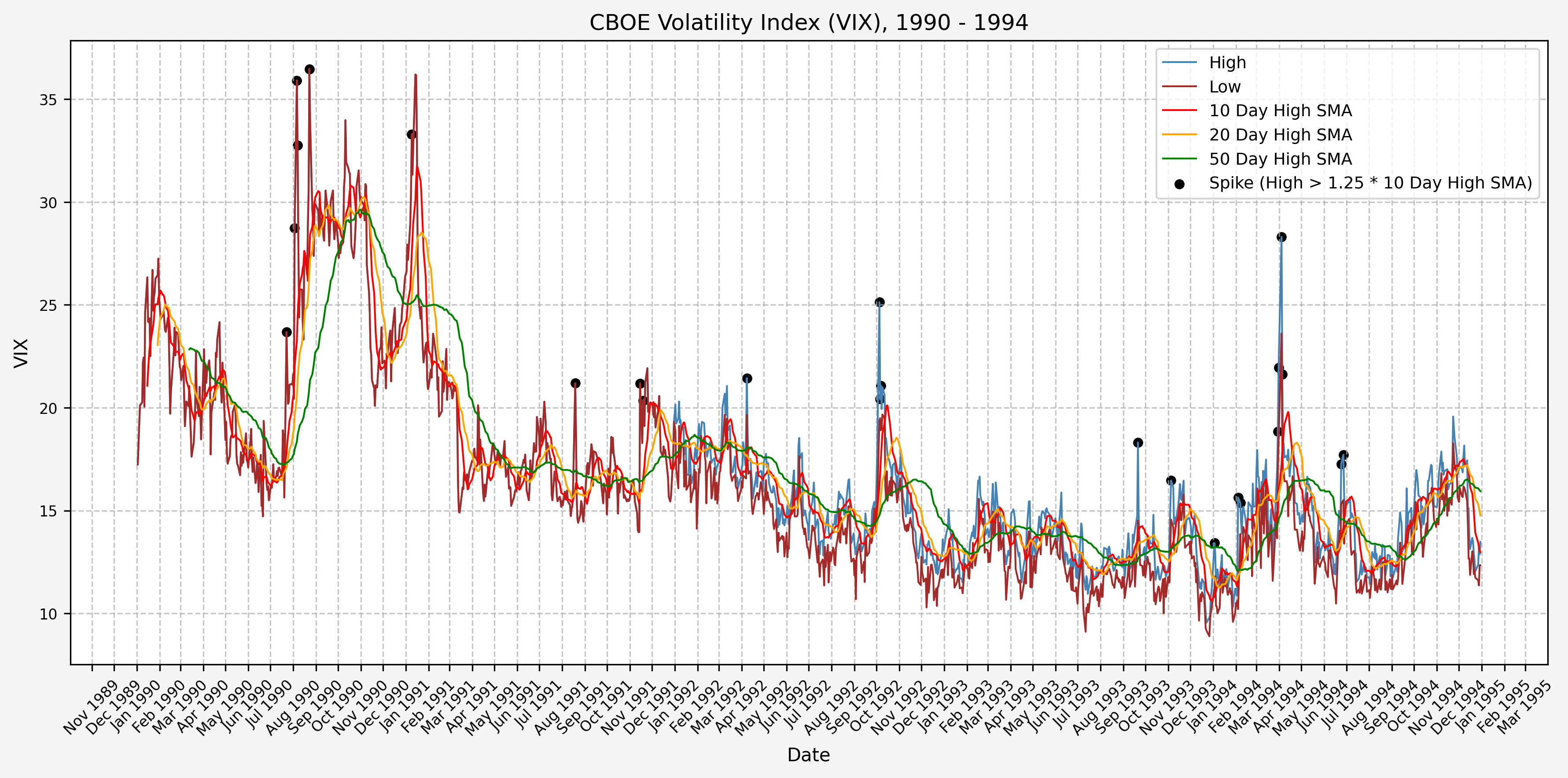
Spike Counts (Signals) Plots By Decade
And here are the plots for the signals generated over the past 3 decades:
1990 - 1994
1995 - 1999
2000 - 2004
2005 - 2009
2010 - 2014
2015 - 2019
2020 - 2024
2025 - Present

Trading History
I’ve begun trading based on the above ideas, opening positions during the VIX spikes and closing them as volatility comes back down. The executed trades, closed positions, and open positions listed below are all automated updates from the transaction history exports from Schwab. The exported CSV files are available in the GitHub repository.
Trades Executed
Here are the trades executed to date:
| Trade_Date | Action | Symbol | Quantity | Price | Fees & Comm | Amount |
|---|
| 2024-08-05 00:00:00 | Buy to Open | VIX 09/18/2024 34.00 P | 1 | 10.95 | 1.08 | 1096.08 |
| 2024-08-21 00:00:00 | Sell to Close | VIX 09/18/2024 34.00 P | 1 | 17.95 | 1.08 | 1793.92 |
| 2024-08-05 00:00:00 | Buy to Open | VIX 10/16/2024 40.00 P | 1 | 16.35 | 1.08 | 1636.08 |
| 2024-09-18 00:00:00 | Sell to Close | VIX 10/16/2024 40.00 P | 1 | 21.54 | 1.08 | 2152.92 |
| 2024-08-07 00:00:00 | Buy to Open | VIX 11/20/2024 25.00 P | 2 | 5.90 | 2.16 | 1182.16 |
| 2024-11-04 00:00:00 | Sell to Close | VIX 11/20/2024 25.00 P | 2 | 6.10 | 2.16 | 1217.84 |
| 2024-08-06 00:00:00 | Buy to Open | VIX 12/18/2024 30.00 P | 1 | 10.25 | 1.08 | 1026.08 |
| 2024-11-27 00:00:00 | Sell to Close | VIX 12/18/2024 30.00 P | 1 | 14.95 | 1.08 | 1493.92 |
| 2025-03-04 00:00:00 | Buy to Open | VIX 04/16/2025 25.00 P | 5 | 5.65 | 5.40 | 2830.40 |
| 2025-03-24 00:00:00 | Sell to Close | VIX 04/16/2025 25.00 P | 5 | 7.00 | 5.40 | 3494.60 |
| 2025-03-10 00:00:00 | Buy to Open | VIX 05/21/2025 26.00 P | 5 | 7.10 | 5.40 | 3555.40 |
| 2025-04-04 00:00:00 | Buy to Open | VIX 05/21/2025 26.00 P | 10 | 4.10 | 10.81 | 4110.81 |
| 2025-04-04 00:00:00 | Buy to Open | VIX 05/21/2025 37.00 P | 3 | 13.20 | 3.24 | 3963.24 |
| 2025-04-08 00:00:00 | Buy to Open | VIX 05/21/2025 50.00 P | 2 | 21.15 | 2.16 | 4232.16 |
| 2025-04-24 00:00:00 | Sell to Close | VIX 05/21/2025 50.00 P | 1 | 25.30 | 1.08 | 2528.92 |
| 2025-04-24 00:00:00 | Sell to Close | VIX 05/21/2025 26.00 P | 7 | 3.50 | 7.57 | 2442.43 |
| 2025-04-25 00:00:00 | Sell to Close | VIX 05/21/2025 50.00 P | 1 | 25.65 | 1.08 | 2563.92 |
| 2025-04-03 00:00:00 | Buy to Open | VIX 06/18/2025 27.00 P | 8 | 7.05 | 8.65 | 5648.65 |
| 2025-04-04 00:00:00 | Buy to Open | VIX 06/18/2025 36.00 P | 3 | 13.40 | 3.24 | 4023.24 |
| 2025-04-07 00:00:00 | Buy to Open | VIX 06/18/2025 45.00 P | 2 | 18.85 | 2.16 | 3772.16 |
| 2025-04-08 00:00:00 | Buy to Open | VIX 06/18/2025 27.00 P | 4 | 4.55 | 4.32 | 1824.32 |
| 2025-04-03 00:00:00 | Buy to Open | VIX 07/16/2025 29.00 P | 5 | 8.55 | 5.40 | 4280.40 |
| 2025-04-04 00:00:00 | Buy to Open | VIX 07/16/2025 36.00 P | 3 | 13.80 | 3.24 | 4143.24 |
| 2025-04-07 00:00:00 | Buy to Open | VIX 07/16/2025 45.00 P | 2 | 21.55 | 2.16 | 4312.16 |
| 2025-04-07 00:00:00 | Buy to Open | VIX 08/20/2025 45.00 P | 2 | 21.75 | 2.16 | 4352.16 |
Closed Positions
Here are the closed positions:
| Symbol | Amount_Buy | Quantity_Buy | Amount_Sell | Quantity_Sell | Realized_PnL | Profit_Percent |
|---|
| VIX 09/18/2024 34.00 P | 1096.08 | 1 | 1793.92 | 1 | 697.84 | 0.64 |
| VIX 10/16/2024 40.00 P | 1636.08 | 1 | 2152.92 | 1 | 516.84 | 0.32 |
| VIX 11/20/2024 25.00 P | 1182.16 | 2 | 1217.84 | 2 | 35.68 | 0.03 |
| VIX 12/18/2024 30.00 P | 1026.08 | 1 | 1493.92 | 1 | 467.84 | 0.46 |
| VIX 04/16/2025 25.00 P | 2830.40 | 5 | 3494.60 | 5 | 664.20 | 0.23 |
| VIX 05/21/2025 50.00 P | 4232.16 | 2 | 5092.84 | 2 | 860.68 | 0.20 |
Net profit and loss percentage: 27.02%Net profit and loss: $3,243.08
Open Positions
Here are the positions that are currently open:
| Symbol | Amount_Buy | Quantity_Buy |
|---|
| VIX 05/21/2025 26.00 P | 7666.21 | 15 |
| VIX 05/21/2025 37.00 P | 3963.24 | 3 |
| VIX 06/18/2025 27.00 P | 7472.97 | 12 |
| VIX 06/18/2025 36.00 P | 4023.24 | 3 |
| VIX 06/18/2025 45.00 P | 3772.16 | 2 |
| VIX 07/16/2025 29.00 P | 4280.40 | 5 |
| VIX 07/16/2025 36.00 P | 4143.24 | 3 |
| VIX 07/16/2025 45.00 P | 4312.16 | 2 |
| VIX 08/20/2025 45.00 P | 4352.16 | 2 |
References
https://www.cboe.com/tradable_products/vix/https://github.com/ranaroussi/yfinance
Code
The jupyter notebook with the functions and all other code is available here.The html export of the jupyter notebook is available here.The pdf export of the jupyter notebook is available here.