Does Harry Browne's permanent portfolio withstand the test of time?

Introduction

Harry Browne was an influencial politician, financial advisor, and author who lived from 1933 to 2006 and published 12 books. Wikipedia has an in-depth biography on him.

Within the world of finance and investing, one of his best known works is Fail-Safe Investing: Lifelong Financial Security in 30 Minutes. In it, he introduces the idea of the “Permanent Portfolio”, an investment strategy that uses only four assets and is very simple to implement.

In this post, we will investigate Browne’s suggested portfolio, including performance across various market cycles and economic regimes.

Browne’s Portfolio Requirements

In Fail-Safe Investing, under rule #11, Browne lays out the requirements for a “bulletproof portfolio” that will “assure that your wealth will survive any event - including events that would be devastating to any one investment. In other words, this portfolio should protect you no matter what the future brings.”

His requirements for the portfolio consist of the followng:

Safety: Protection again any economic future, including “inflation, recession, or even depression”
Stability: Performance should be consistent so that you will not need to make any changes and will not experience significant drawdowns
Simplicity: Easy to implement and take very little time to maintain

He then describes the four “broad movements” of the economy:

Prosperity: The economy is growing, business is doing well, interest rates are usually low
Inflation: The cost of goods and services is rising
Tight money or recession: The money supply is shrinking, economic activity is slowing
Deflation: Prices are declining and the value of money is increasing

The Permanent Portfolio

Browne then matches an asset class to each of the economic conditions above:

Prosperity -> Stocks (due to prosperity) and long term bonds (when interest rates fall)
Inflation -> Gold
Deflation -> Long term bonds (when interest rates fall)
Tight money -> Cash

He completes the Permanent Portfolio by stipulating the following:

Start with a base allocation of 25% to each of the asset classes (stocks, bonds, gold, cash)
Rebalance back to the base allocation annually, or when “any of the four investments has become worth less than 15%, or more than 35%, of the portfolio’s overall value”
Note: Browne does not specify when the portfolio should be rebalanced; therefore, we will make an assumption of a January 1st rebalance.

Data

For this exercise, we will use the following asset classes:

Stocks: S&P 500 (SPXT_S&P 500 Total Return Index)
Bonds: 10 Year US Treasuries (SPBDU10T_S&P US Treasury Bond 7-10 Year Total Return Index)
Gold: Gold Spot Price (XAU_Gold USD Spot)
Cash: USD

With the exception of cash, all data is sourced from Bloomberg.

We could use ETFs, but the available price history for the ETFs is much shorter than the indices above. If we wanted to use ETFs, the following would work:

Stocks: IVV - iShares Core S&P 500 ETF
Bonds: IEF - iShares 7-10 Year Treasury Bond ETF
Gold: IAU - iShares Gold Trust
Cash: USD

Python Functions

Here are the functions needed for this project:

bb_clean_data: Takes an Excel export from Bloomberg, removes the miscellaneous headings/rows, and returns a DataFrame.
df_info: A simple function to display the information about a DataFrame and the first five rows and last five rows.
df_info_markdown: Similar to the df_info function above, except that it coverts the output to markdown.
export_track_md_deps: Exports various text outputs to markdown files, which are included in the index.md file created when building the site with Hugo.
load_data: Load data from a CSV, Excel, or Pickle file into a pandas DataFrame.
pandas_set_decimal_places: Set the number of decimal places displayed for floating-point numbers in pandas.
strategy_harry_brown_perm_port: Execute the strategy for the Harry Brown permanent portfolio.
summary_stats: Generate summary statistics for a series of returns.

Data Overview

Load Data

As previously mentioned, the data for this exercise comes primarily from Bloomberg. We’ll start with loading the data first for bonds:

 1
 2
 3
 4
 5
 6
 7
 8
 9
10
11
12
13
14
15
16
17
18
19
20
21
22
23
24
25
26
27
28
29
# Set decimal places
pandas_set_decimal_places(3)

# Bonds dataframe
bb_clean_data(
    base_directory=DATA_DIR,
    fund_ticker_name="SPBDU10T_S&P US Treasury Bond 7-10 Year Total Return Index",
    source="Bloomberg",
    asset_class="Indices",
    excel_export=True,
    pickle_export=True,
    output_confirmation=True,
)

bonds_data = load_data(
    base_directory=DATA_DIR,
    ticker="SPBDU10T_S&P US Treasury Bond 7-10 Year Total Return Index_Clean",
    source="Bloomberg",
    asset_class="Indices",
    timeframe="Daily",
)

bonds_data['Date'] = pd.to_datetime(bonds_data['Date'])
bonds_data.set_index('Date', inplace = True)
bonds_data = bonds_data[(bonds_data.index >= '1990-01-01') & (bonds_data.index <= '2023-12-31')]
bonds_data.rename(columns={'Close':'Bonds_Close'}, inplace=True)
bonds_data['Bonds_Daily_Return'] = bonds_data['Bonds_Close'].pct_change()
bonds_data['Bonds_Total_Return'] = (1 + bonds_data['Bonds_Daily_Return']).cumprod()
display(bonds_data.head())

The following is the output:

Date	Bonds_Close	Bonds_Daily_Return	Bonds_Total_Return
1990-01-02 00:00:00	99.972	nan	nan
1990-01-03 00:00:00	99.733	-0.002	0.998
1990-01-04 00:00:00	99.813	0.001	0.998
1990-01-05 00:00:00	99.769	-0.000	0.998
1990-01-08 00:00:00	99.681	-0.001	0.997

Then for stocks:

 1
 2
 3
 4
 5
 6
 7
 8
 9
10
11
12
13
14
15
16
17
18
19
20
21
22
23
24
25
26
# Stocks dataframe
bb_clean_data(
    base_directory=DATA_DIR,
    fund_ticker_name="SPXT_S&P 500 Total Return Index",
    source="Bloomberg",
    asset_class="Indices",
    excel_export=True,
    pickle_export=True,
    output_confirmation=True,
)

stocks_data = load_data(
    base_directory=DATA_DIR,
    ticker="SPXT_S&P 500 Total Return Index_Clean",
    source="Bloomberg",
    asset_class="Indices",
    timeframe="Daily",
)

stocks_data['Date'] = pd.to_datetime(stocks_data['Date'])
stocks_data.set_index('Date', inplace = True)
stocks_data = stocks_data[(stocks_data.index >= '1990-01-01') & (stocks_data.index <= '2023-12-31')]
stocks_data.rename(columns={'Close':'Stocks_Close'}, inplace=True)
stocks_data['Stocks_Daily_Return'] = stocks_data['Stocks_Close'].pct_change()
stocks_data['Stocks_Total_Return'] = (1 + stocks_data['Stocks_Daily_Return']).cumprod()
display(stocks_data.head())

The following is the output:

Date	Stocks_Close	Stocks_Daily_Return	Stocks_Total_Return
1990-01-01 00:00:00	nan	nan	nan
1990-01-02 00:00:00	386.160	nan	nan
1990-01-03 00:00:00	385.170	-0.003	0.997
1990-01-04 00:00:00	382.020	-0.008	0.989
1990-01-05 00:00:00	378.300	-0.010	0.980

And finally, gold:

 1
 2
 3
 4
 5
 6
 7
 8
 9
10
11
12
13
14
15
16
17
18
19
20
21
22
23
24
25
26
# Gold dataframe
bb_clean_data(
    base_directory=DATA_DIR,
    fund_ticker_name="XAU_Gold USD Spot",
    source="Bloomberg",
    asset_class="Commodities",
    excel_export=True,
    pickle_export=True,
    output_confirmation=True,
)

gold_data = load_data(
    base_directory=DATA_DIR,
    ticker="XAU_Gold USD Spot_Clean",
    source="Bloomberg",
    asset_class="Commodities",
    timeframe="Daily",
)

gold_data['Date'] = pd.to_datetime(gold_data['Date'])
gold_data.set_index('Date', inplace = True)
gold_data = gold_data[(gold_data.index >= '1990-01-01') & (gold_data.index <= '2023-12-31')]
gold_data.rename(columns={'Close':'Gold_Close'}, inplace=True)
gold_data['Gold_Daily_Return'] = gold_data['Gold_Close'].pct_change()
gold_data['Gold_Total_Return'] = (1 + gold_data['Gold_Daily_Return']).cumprod()
display(gold_data.head())

The following is the output:

Date	Gold_Close	Gold_Daily_Return	Gold_Total_Return
1990-01-02 00:00:00	399.000	nan	nan
1990-01-03 00:00:00	395.000	-0.010	0.990
1990-01-04 00:00:00	396.500	0.004	0.994
1990-01-05 00:00:00	405.000	0.021	1.015
1990-01-08 00:00:00	404.600	-0.001	1.014

Combine Data

We’ll now combine the dataframes for the timeseries data from each of the asset classes, as follows:

 1
 2
 3
 4
 5
 6
 7
 8
 9
10
11
12
13
14
# Merge the stock data and bond data into a single DataFrame using their indices (dates)
perm_port = pd.merge(stocks_data['Stocks_Close'], bonds_data['Bonds_Close'], left_index=True, right_index=True)

# Add gold data to the portfolio DataFrame by merging it with the existing data on indices (dates)
perm_port = pd.merge(perm_port, gold_data['Gold_Close'], left_index=True, right_index=True)

# Add a column for cash with a constant value of 1 (assumes the value of cash remains constant at $1 over time)
perm_port['Cash_Close'] = 1

# Remove any rows with missing values (NaN) to ensure clean data for further analysis
perm_port.dropna(inplace=True)

# Display the finalized portfolio DataFrame
display(perm_port)

Check For Missing Values

We can check for any missing (NaN) values in each column:

1
2
# Check for any missing values in each column
perm_port.isnull().any()

DataFrame Info

Now, running:

1
df_info(perm_port)

Gives us the following:

 1
 2
 3
 4
 5
 6
 7
 8
 9
10
11
12
13
The columns, shape, and data types are:

<class 'pandas.core.frame.DataFrame'>
DatetimeIndex: 8479 entries, 1990-01-02 to 2023-12-29
Data columns (total 4 columns):
 #   Column        Non-Null Count  Dtype  
---  ------        --------------  -----  
 0   Stocks_Close  8479 non-null   float64
 1   Bonds_Close   8479 non-null   float64
 2   Gold_Close    8479 non-null   float64
 3   Cash_Close    8479 non-null   int64  
dtypes: float64(3), int64(1)
memory usage: 331.2 KB

The first 5 rows are:

Date	Stocks_Close	Bonds_Close	Gold_Close	Cash_Close
1990-01-02 00:00:00	386.16	99.97	399.00	1.00
1990-01-03 00:00:00	385.17	99.73	395.00	1.00
1990-01-04 00:00:00	382.02	99.81	396.50	1.00
1990-01-05 00:00:00	378.30	99.77	405.00	1.00
1990-01-08 00:00:00	380.04	99.68	404.60	1.00

The last 5 rows are:

Date	Stocks_Close	Bonds_Close	Gold_Close	Cash_Close
2023-12-22 00:00:00	10292.37	604.17	2053.08	1.00
2023-12-26 00:00:00	10335.98	604.55	2067.81	1.00
2023-12-27 00:00:00	10351.60	609.36	2077.49	1.00
2023-12-28 00:00:00	10356.59	606.83	2065.61	1.00
2023-12-29 00:00:00	10327.83	606.18	2062.98	1.00

We can see that we have daily close price data for all 4 asset classes from the beginning of 1990 to the end of 2023.

Execute Strategy

Using an annual rebalance date of January 1, we’ll now execute the strategy with the following code:

 1
 2
 3
 4
 5
 6
 7
 8
 9
10
11
12
13
14
15
16
17
18
19
20
21
22
23
24
# List of funds to be used
fund_list = ['Stocks', 'Bonds', 'Gold', 'Cash']

# Starting cash contribution
starting_cash = 10000

# Monthly cash contribution
cash_contrib = 0

strat = strategy_harry_brown_perm_port(
    fund_list=fund_list, 
    starting_cash=starting_cash, 
    cash_contrib=cash_contrib, 
    close_prices_df=perm_port, 
    rebal_month=1, 
    rebal_day=1, 
    rebal_per_high=0.35, 
    rebal_per_low=0.15,
    excel_export=True,
    pickle_export=True,
    output_confirmation=True,
)

strat = strat.set_index('Date')

This returns a dataframe with the entire strategy.

Running:

1
df_info(strat)

Gives us:

 1
 2
 3
 4
 5
 6
 7
 8
 9
10
11
12
13
14
15
16
17
18
19
20
21
22
23
24
25
26
27
28
29
30
31
32
33
34
35
36
37
38
39
40
41
42
43
The columns, shape, and data types are:

<class 'pandas.core.frame.DataFrame'>
DatetimeIndex: 8479 entries, 1990-01-02 to 2023-12-29
Data columns (total 34 columns):
 #   Column                Non-Null Count  Dtype  
---  ------                --------------  -----  
 0   Stocks_Close          8479 non-null   float64
 1   Bonds_Close           8479 non-null   float64
 2   Gold_Close            8479 non-null   float64
 3   Cash_Close            8479 non-null   int64  
 4   Stocks_BA_Shares      8479 non-null   float64
 5   Stocks_BA_$_Invested  8479 non-null   float64
 6   Stocks_BA_Port_%      8479 non-null   float64
 7   Bonds_BA_Shares       8479 non-null   float64
 8   Bonds_BA_$_Invested   8479 non-null   float64
 9   Bonds_BA_Port_%       8479 non-null   float64
 10  Gold_BA_Shares        8479 non-null   float64
 11  Gold_BA_$_Invested    8479 non-null   float64
 12  Gold_BA_Port_%        8479 non-null   float64
 13  Cash_BA_Shares        8479 non-null   float64
 14  Cash_BA_$_Invested    8479 non-null   float64
 15  Cash_BA_Port_%        8479 non-null   float64
 16  Total_BA_$_Invested   8479 non-null   float64
 17  Contribution          8479 non-null   int64  
 18  Rebalance             8479 non-null   object 
 19  Stocks_AA_Shares      8479 non-null   float64
 20  Stocks_AA_$_Invested  8479 non-null   float64
 21  Stocks_AA_Port_%      8479 non-null   float64
 22  Bonds_AA_Shares       8479 non-null   float64
 23  Bonds_AA_$_Invested   8479 non-null   float64
 24  Bonds_AA_Port_%       8479 non-null   float64
 25  Gold_AA_Shares        8479 non-null   float64
 26  Gold_AA_$_Invested    8479 non-null   float64
 27  Gold_AA_Port_%        8479 non-null   float64
 28  Cash_AA_Shares        8479 non-null   float64
 29  Cash_AA_$_Invested    8479 non-null   float64
 30  Cash_AA_Port_%        8479 non-null   float64
 31  Total_AA_$_Invested   8479 non-null   float64
 32  Return                8478 non-null   float64
 33  Cumulative_Return     8478 non-null   float64
dtypes: float64(31), int64(2), object(1)
memory usage: 2.3+ MB

The first 5 rows are:

Date	Stocks_Close	Bonds_Close	Gold_Close	Cash_Close	Stocks_BA_Shares	Stocks_BA_$_Invested	Stocks_BA_Port_%	Bonds_BA_Shares	Bonds_BA_$_Invested	Bonds_BA_Port_%	Gold_BA_Shares	Gold_BA_$_Invested	Gold_BA_Port_%	Cash_BA_Shares	Cash_BA_$_Invested	Cash_BA_Port_%	Total_BA_$_Invested	Rebalance	Stocks_AA_Shares	Stocks_AA_$_Invested	Stocks_AA_Port_%	Bonds_AA_Shares	Bonds_AA_$_Invested	Bonds_AA_Port_%	Gold_AA_Shares	Gold_AA_$_Invested	Gold_AA_Port_%	Cash_AA_Shares	Cash_AA_$_Invested	Cash_AA_Port_%	Total_AA_$_Invested	Return	Cumulative_Return
1990-01-02 00:00:00	386.16	99.97	399.00	1	6.47	2500.00	0.25	25.01	2500.00	0.25	6.27	2500.00	0.25	2500.00	2500.00	0.25	10000.00	No	6.47	2500.00	0.25	25.01	2500.00	0.25	6.27	2500.00	0.25	2500.00	2500.00	0.25	10000.00	nan	nan
1990-01-03 00:00:00	385.17	99.73	395.00	1	6.47	2493.59	0.25	25.01	2494.02	0.25	6.27	2474.94	0.25	2500.00	2500.00	0.25	9962.55	No	6.47	2493.59	0.25	25.01	2494.02	0.25	6.27	2474.94	0.25	2500.00	2500.00	0.25	9962.55	-0.00	1.00
1990-01-04 00:00:00	382.02	99.81	396.50	1	6.47	2473.20	0.25	25.01	2496.02	0.25	6.27	2484.34	0.25	2500.00	2500.00	0.25	9953.56	No	6.47	2473.20	0.25	25.01	2496.02	0.25	6.27	2484.34	0.25	2500.00	2500.00	0.25	9953.56	-0.00	1.00
1990-01-05 00:00:00	378.30	99.77	405.00	1	6.47	2449.11	0.25	25.01	2494.92	0.25	6.27	2537.59	0.25	2500.00	2500.00	0.25	9981.63	No	6.47	2449.11	0.25	25.01	2494.92	0.25	6.27	2537.59	0.25	2500.00	2500.00	0.25	9981.63	0.00	1.00
1990-01-08 00:00:00	380.04	99.68	404.60	1	6.47	2460.38	0.25	25.01	2492.72	0.25	6.27	2535.09	0.25	2500.00	2500.00	0.25	9988.19	No	6.47	2460.38	0.25	25.01	2492.72	0.25	6.27	2535.09	0.25	2500.00	2500.00	0.25	9988.19	0.00	1.00

The last 5 rows are:

Date	Stocks_Close	Bonds_Close	Gold_Close	Cash_Close	Stocks_BA_Shares	Stocks_BA_$_Invested	Stocks_BA_Port_%	Bonds_BA_Shares	Bonds_BA_$_Invested	Bonds_BA_Port_%	Gold_BA_Shares	Gold_BA_$_Invested	Gold_BA_Port_%	Cash_BA_Shares	Cash_BA_$_Invested	Cash_BA_Port_%	Total_BA_$_Invested	Rebalance	Stocks_AA_Shares	Stocks_AA_$_Invested	Stocks_AA_Port_%	Bonds_AA_Shares	Bonds_AA_$_Invested	Bonds_AA_Port_%	Gold_AA_Shares	Gold_AA_$_Invested	Gold_AA_Port_%	Cash_AA_Shares	Cash_AA_$_Invested	Cash_AA_Port_%	Total_AA_$_Invested	Return	Cumulative_Return
2023-12-22 00:00:00	10292.37	604.17	2053.08	1	1.81	18595.87	0.29	25.03	15124.46	0.23	8.00	16426.12	0.25	14717.17	14717.17	0.23	64863.62	No	1.81	18595.87	0.29	25.03	15124.46	0.23	8.00	16426.12	0.25	14717.17	14717.17	0.23	64863.62	0.00	6.49
2023-12-26 00:00:00	10335.98	604.55	2067.81	1	1.81	18674.66	0.29	25.03	15134.20	0.23	8.00	16543.97	0.25	14717.17	14717.17	0.23	65070.01	No	1.81	18674.66	0.29	25.03	15134.20	0.23	8.00	16543.97	0.25	14717.17	14717.17	0.23	65070.01	0.00	6.51
2023-12-27 00:00:00	10351.60	609.36	2077.49	1	1.81	18702.89	0.29	25.03	15254.36	0.23	8.00	16621.42	0.25	14717.17	14717.17	0.23	65295.84	No	1.81	18702.89	0.29	25.03	15254.36	0.23	8.00	16621.42	0.25	14717.17	14717.17	0.23	65295.84	0.00	6.53
2023-12-28 00:00:00	10356.59	606.83	2065.61	1	1.81	18711.90	0.29	25.03	15191.10	0.23	8.00	16526.37	0.25	14717.17	14717.17	0.23	65146.54	No	1.81	18711.90	0.29	25.03	15191.10	0.23	8.00	16526.37	0.25	14717.17	14717.17	0.23	65146.54	-0.00	6.51
2023-12-29 00:00:00	10327.83	606.18	2062.98	1	1.81	18659.94	0.29	25.03	15175.01	0.23	8.00	16505.33	0.25	14717.17	14717.17	0.23	65057.44	No	1.81	18659.94	0.29	25.03	15175.01	0.23	8.00	16505.33	0.25	14717.17	14717.17	0.23	65057.44	-0.00	6.51

From the above, we can see that there are all columns for before/after re-balancing, including the shares, asset values, percentages, etc. for the four different asset classes.

Strategy Statistics

Let’s look at the summary statistics for the entire timeframe, as well as several different ranges:

 1
 2
 3
 4
 5
 6
 7
 8
 9
10
11
12
13
14
15
16
17
18
19
20
21
22
23
24
25
26
27
28
29
30
31
32
33
34
35
36
37
38
sum_stats = summary_stats(
    fund_list=fund_list,
    df=strat[['Return']],
    period="Daily",
    excel_export=True,
    pickle_export=True,
    output_confirmation=True,
)

strat_pre_1999 = strat[strat.index < '2000-01-01']
sum_stats_pre_1999 = summary_stats(
    fund_list=fund_list, 
    df=strat_pre_1999[['Return']], 
    period="Daily",
    excel_export=False,
    pickle_export=False,
    output_confirmation=True,
)

strat_post_1999 = strat[strat.index >= '2000-01-01']
sum_stats_post_1999 = summary_stats(
    fund_list=fund_list, 
    df=strat_post_1999[['Return']], 
    period="Daily",
    excel_export=False,
    pickle_export=False,
    output_confirmation=True,
)

strat_post_2009 = strat[strat.index >= '2010-01-01']
sum_stats_post_2009 = summary_stats(
    fund_list=fund_list, 
    df=strat_post_2009[['Return']], 
    period="Daily",
    excel_export=False,
    pickle_export=False,
    output_confirmation=True,
)

And the concat them to make comparing them easier:

1
2
3
4
5
6
7
8
9
all_sum_stats = pd.concat([sum_stats])
all_sum_stats = all_sum_stats.rename(index={'Return': '1990 - 2023'})
all_sum_stats = pd.concat([all_sum_stats, sum_stats_pre_1999])
all_sum_stats = all_sum_stats.rename(index={'Return': 'Pre 1999'})
all_sum_stats = pd.concat([all_sum_stats, sum_stats_post_1999])
all_sum_stats = all_sum_stats.rename(index={'Return': 'Post 1999'})
all_sum_stats = pd.concat([all_sum_stats, sum_stats_post_2009])
all_sum_stats = all_sum_stats.rename(index={'Return': 'Post 2009'})
display(all_sum_stats)

Which gives us:

	Annualized Mean	Annualized Volatility	Annualized Sharpe Ratio	CAGR	Daily Max Return	Daily Max Return (Date)	Daily Min Return	Daily Min Return (Date)	Max Drawdown	Peak	Bottom	Recovery Date
1990 - 2023	0.057	0.060	0.957	0.057	0.029	2020-03-24 00:00:00	-0.030	2020-03-12 00:00:00	-0.154	2008-03-18 00:00:00	2008-11-12 00:00:00	2009-10-06 00:00:00
Pre 1999	0.060	0.050	1.207	0.061	0.022	1999-09-28 00:00:00	-0.018	1993-08-05 00:00:00	-0.062	1998-07-20 00:00:00	1998-08-31 00:00:00	1998-11-05 00:00:00
Post 1999	0.056	0.064	0.883	0.056	0.029	2020-03-24 00:00:00	-0.030	2020-03-12 00:00:00	-0.154	2008-03-18 00:00:00	2008-11-12 00:00:00	2009-10-06 00:00:00
Post 2009	0.056	0.060	0.927	0.056	0.029	2020-03-24 00:00:00	-0.030	2020-03-12 00:00:00	-0.127	2021-12-27 00:00:00	2022-10-20 00:00:00	2023-12-01 00:00:00

Annual Returns

Here’s the annual returns:

Year	Return
1991	0.102
1992	0.030
1993	0.099
1994	-0.017
1995	0.153
1996	0.049
1997	0.056
1998	0.102
1999	0.039
2000	0.000
2001	-0.005
2002	0.043
2003	0.121
2004	0.051
2005	0.064
2006	0.104
2007	0.117
2008	-0.033
2009	0.107
2010	0.137
2011	0.070
2012	0.068
2013	-0.006
2014	0.052
2015	-0.018
2016	0.052
2017	0.095
2018	-0.012
2019	0.145
2020	0.134
2021	0.057
2022	-0.082
2023	0.109

Since the strategy, summary statistics, and annual returns are all exported as excel files, they can be found at the following locations:

Next we will look at some plots to help visualize the data.

Generate Plots

Here are the various functions needed for the plots:

Plot Cumulative Return

Plot cumulative return:

 1
 2
 3
 4
 5
 6
 7
 8
 9
10
11
12
13
14
15
16
17
18
19
20
21
22
23
24
25
26
27
28
29
30
31
32
33
34
35
36
def plot_cumulative_return(strat_df):
    # Generate plot
    plt.figure(figsize=(10, 5), facecolor = '#F5F5F5')

    # Plotting data
    plt.plot(strat_df.index, strat_df['Cumulative_Return'], label = 'Strategy Cumulative Return', linestyle='-', color='green', linewidth=1)
    
    # Set X axis
    # x_tick_spacing = 5  # Specify the interval for x-axis ticks
    # plt.gca().xaxis.set_major_locator(MultipleLocator(x_tick_spacing))
    plt.gca().xaxis.set_major_locator(mdates.YearLocator())
    plt.gca().xaxis.set_major_formatter(mdates.DateFormatter('%Y'))
    plt.xlabel('Year', fontsize = 9)
    plt.xticks(rotation = 45, fontsize = 7)
    # plt.xlim(, )

    # Set Y axis
    y_tick_spacing = 0.5  # Specify the interval for y-axis ticks
    plt.gca().yaxis.set_major_locator(MultipleLocator(y_tick_spacing))
    plt.ylabel('Cumulative Return', fontsize = 9)
    plt.yticks(fontsize = 7)
    plt.ylim(0, 7.5)

    # Set title, etc.
    plt.title('Cumulative Return', fontsize = 12)
    
    # Set the grid & legend
    plt.tight_layout()
    plt.grid(True)
    plt.legend(fontsize=8)

    # Save the figure
    plt.savefig('03_Cumulative_Return.png', dpi=300, bbox_inches='tight')

    # Display the plot
    return plt.show()

Plot Portfolio Values

Plot portfolio values:

 1
 2
 3
 4
 5
 6
 7
 8
 9
10
11
12
13
14
15
16
17
18
19
20
21
22
23
24
25
26
27
28
29
30
31
32
33
34
35
36
37
38
39
40
41
42
def plot_values(strat_df):   
    # Generate plot   
    plt.figure(figsize=(10, 5), facecolor = '#F5F5F5')
    
    # Plotting data
    plt.plot(strat_df.index, strat_df['Total_AA_$_Invested'], label='Total Portfolio Value', linestyle='-', color='black', linewidth=1)
    plt.plot(strat_df.index, strat_df['Stocks_AA_$_Invested'], label='Stocks Position Value', linestyle='-', color='orange', linewidth=1)
    plt.plot(strat_df.index, strat_df['Bonds_AA_$_Invested'], label='Bond Position Value', linestyle='-', color='yellow', linewidth=1)
    plt.plot(strat_df.index, strat_df['Gold_AA_$_Invested'], label='Gold Position Value', linestyle='-', color='blue', linewidth=1)
    plt.plot(strat_df.index, strat_df['Cash_AA_$_Invested'], label='Cash Position Value', linestyle='-', color='brown', linewidth=1)

    # Set X axis
    # x_tick_spacing = 5  # Specify the interval for x-axis ticks
    # plt.gca().xaxis.set_major_locator(MultipleLocator(x_tick_spacing))
    plt.gca().xaxis.set_major_locator(mdates.YearLocator())
    plt.gca().xaxis.set_major_formatter(mdates.DateFormatter('%Y'))
    plt.xlabel('Year', fontsize = 9)
    plt.xticks(rotation = 45, fontsize = 7)
    # plt.xlim(, )


    # Set Y axis
    y_tick_spacing = 5000  # Specify the interval for y-axis ticks
    plt.gca().yaxis.set_major_locator(MultipleLocator(y_tick_spacing))
    plt.gca().yaxis.set_major_formatter(mtick.FuncFormatter(lambda x, pos: '{:,.0f}'.format(x))) # Adding commas to y-axis labels
    plt.ylabel('Total Value ($)', fontsize = 9)
    plt.yticks(fontsize = 7)
    plt.ylim(0, 75000)

    # Set title, etc.
    plt.title('Total Values For Stocks, Bonds, Gold, and Cash Positions and Portfolio', fontsize = 12)
    
    # Set the grid & legend
    plt.tight_layout()
    plt.grid(True)
    plt.legend(fontsize=8)

    # Save the figure
    plt.savefig('04_Portfolio_Values.png', dpi=300, bbox_inches='tight')

    # Display the plot
    return plt.show()

Plot Portfolio Drawdown

Plot portfolio drawdown:

 1
 2
 3
 4
 5
 6
 7
 8
 9
10
11
12
13
14
15
16
17
18
19
20
21
22
23
24
25
26
27
28
29
30
31
32
33
34
35
36
37
38
39
40
41
def plot_drawdown(strat_df):
    rolling_max = strat_df['Total_AA_$_Invested'].cummax()
    drawdown = (strat_df['Total_AA_$_Invested'] - rolling_max) / rolling_max * 100

    # Generate plot   
    plt.figure(figsize=(10, 5), facecolor = '#F5F5F5')

    # Plotting data
    plt.plot(strat_df.index, drawdown, label='Drawdown', linestyle='-', color='red', linewidth=1)
    
    # Set X axis
    # x_tick_spacing = 5  # Specify the interval for x-axis ticks
    # plt.gca().xaxis.set_major_locator(MultipleLocator(x_tick_spacing))
    plt.gca().xaxis.set_major_locator(mdates.YearLocator())
    plt.gca().xaxis.set_major_formatter(mdates.DateFormatter('%Y'))
    plt.xlabel('Year', fontsize = 9)
    plt.xticks(rotation = 45, fontsize = 7)
    # plt.xlim(, )

    # Set Y axis
    y_tick_spacing = 1  # Specify the interval for y-axis ticks
    plt.gca().yaxis.set_major_locator(MultipleLocator(y_tick_spacing))
    # plt.gca().yaxis.set_major_formatter(mtick.FuncFormatter(lambda x, pos: '{:,.0f}'.format(x))) # Adding commas to y-axis labels
    plt.gca().yaxis.set_major_formatter(mtick.FuncFormatter(lambda x, pos: '{:.0f}'.format(x))) # Adding 0 decimal places to y-axis labels
    plt.ylabel('Drawdown (%)', fontsize = 9)
    plt.yticks(fontsize = 7)
    plt.ylim(-20, 0)

    # Set title, etc.
    plt.title('Portfolio Drawdown', fontsize = 12)
    
    # Set the grid & legend
    plt.tight_layout()
    plt.grid(True)
    plt.legend(fontsize=8)

    # Save the figure
    plt.savefig('05_Portfolio_Drawdown.png', dpi=300, bbox_inches='tight')

    # Display the plot
    return plt.show()

Plot Portfolio Asset Weights

Plot portfolio asset weights:

 1
 2
 3
 4
 5
 6
 7
 8
 9
10
11
12
13
14
15
16
17
18
19
20
21
22
23
24
25
26
27
28
29
30
31
32
33
34
35
36
37
38
39
40
def plot_asset_weights(strat_df):
    # Generate plot   
    plt.figure(figsize=(10, 5), facecolor = '#F5F5F5')
    
    # Plotting data
    plt.plot(strat_df.index, strat_df['Stocks_AA_Port_%'] * 100, label='Stocks Portfolio Weight', linestyle='-', color='orange', linewidth=1)
    plt.plot(strat_df.index, strat_df['Bonds_AA_Port_%'] * 100, label='Bonds Portfolio Weight', linestyle='-', color='yellow', linewidth=1)
    plt.plot(strat_df.index, strat_df['Gold_AA_Port_%'] * 100, label='Gold Portfolio Weight', linestyle='-', color='blue', linewidth=1)
    plt.plot(strat_df.index, strat_df['Cash_AA_Port_%'] * 100, label='Cash Portfolio Weight', linestyle='-', color='brown', linewidth=1)

    # Set X axis
    # x_tick_spacing = 5  # Specify the interval for x-axis ticks
    # plt.gca().xaxis.set_major_locator(MultipleLocator(x_tick_spacing))
    plt.gca().xaxis.set_major_locator(mdates.YearLocator())
    plt.gca().xaxis.set_major_formatter(mdates.DateFormatter('%Y'))
    plt.xlabel('Year', fontsize = 9)
    plt.xticks(rotation = 45, fontsize = 7)
    # plt.xlim(, )

    # Set Y axis
    y_tick_spacing = 2  # Specify the interval for y-axis ticks
    plt.gca().yaxis.set_major_locator(MultipleLocator(y_tick_spacing))
    # plt.gca().yaxis.set_major_formatter(mtick.FuncFormatter(lambda x, pos: '{:,.0f}'.format(x))) # Adding commas to y-axis labels
    plt.ylabel('Asset Weight (%)', fontsize = 9)
    plt.yticks(fontsize = 7)
    plt.ylim(14, 36)

    # Set title, etc.
    plt.title('Portfolio Asset Weights For Stocks, Bonds, Gold, and Cash Positions', fontsize = 12)
    
    # Set the grid & legend
    plt.tight_layout()
    plt.grid(True)
    plt.legend(fontsize=8)

    # Save the figure
    plt.savefig('07_Portfolio_Weights.png', dpi=300, bbox_inches='tight')

    # Display the plot
    return plt.show()

Execute plots:

 1
 2
 3
 4
 5
 6
 7
 8
 9
10
11
12
13
14
15
16
17
18
19
20
21
22
23
plot_cumulative_return(strat)
plot_values(strat)
plot_drawdown(strat)
plot_asset_weights(strat)

# Create dataframe for the annual returns
strat_annual_returns = strat['Cumulative_Return'].resample('Y').last().pct_change().dropna()
strat_annual_returns_df = strat_annual_returns.to_frame()
strat_annual_returns_df['Year'] = strat_annual_returns_df.index.year  # Add a 'Year' column with just the year
strat_annual_returns_df.reset_index(drop=True, inplace=True)  # Reset the index to remove the datetime index

# Now the DataFrame will have 'Year' and 'Cumulative_Return' columns
strat_annual_returns_df = strat_annual_returns_df[['Year', 'Cumulative_Return']]  # Keep only 'Year' and 'Cumulative_Return' columns
strat_annual_returns_df.rename(columns = {'Cumulative_Return':'Return'}, inplace=True)
strat_annual_returns_df.set_index('Year', inplace=True)
display(strat_annual_returns_df)

plan_name = '_'.join(fund_list)
file = plan_name + "_Annual_Returns.xlsx"
location = file
strat_annual_returns_df.to_excel(location, sheet_name='data')

plot_annual_returns(strat_annual_returns_df)

Here are several relevant plots:

Cumulative Return

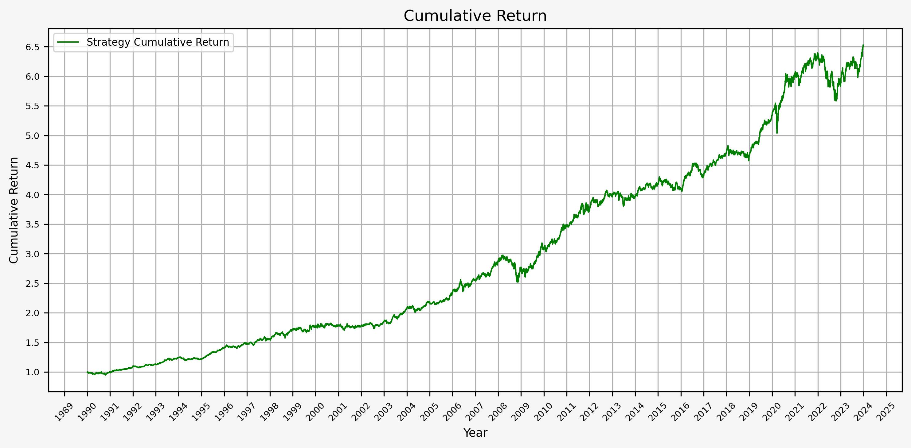
Cumulative Return

Portfolio Values (Total, Stocks, Bonds, Gold, and Cash)

Portfolio Values

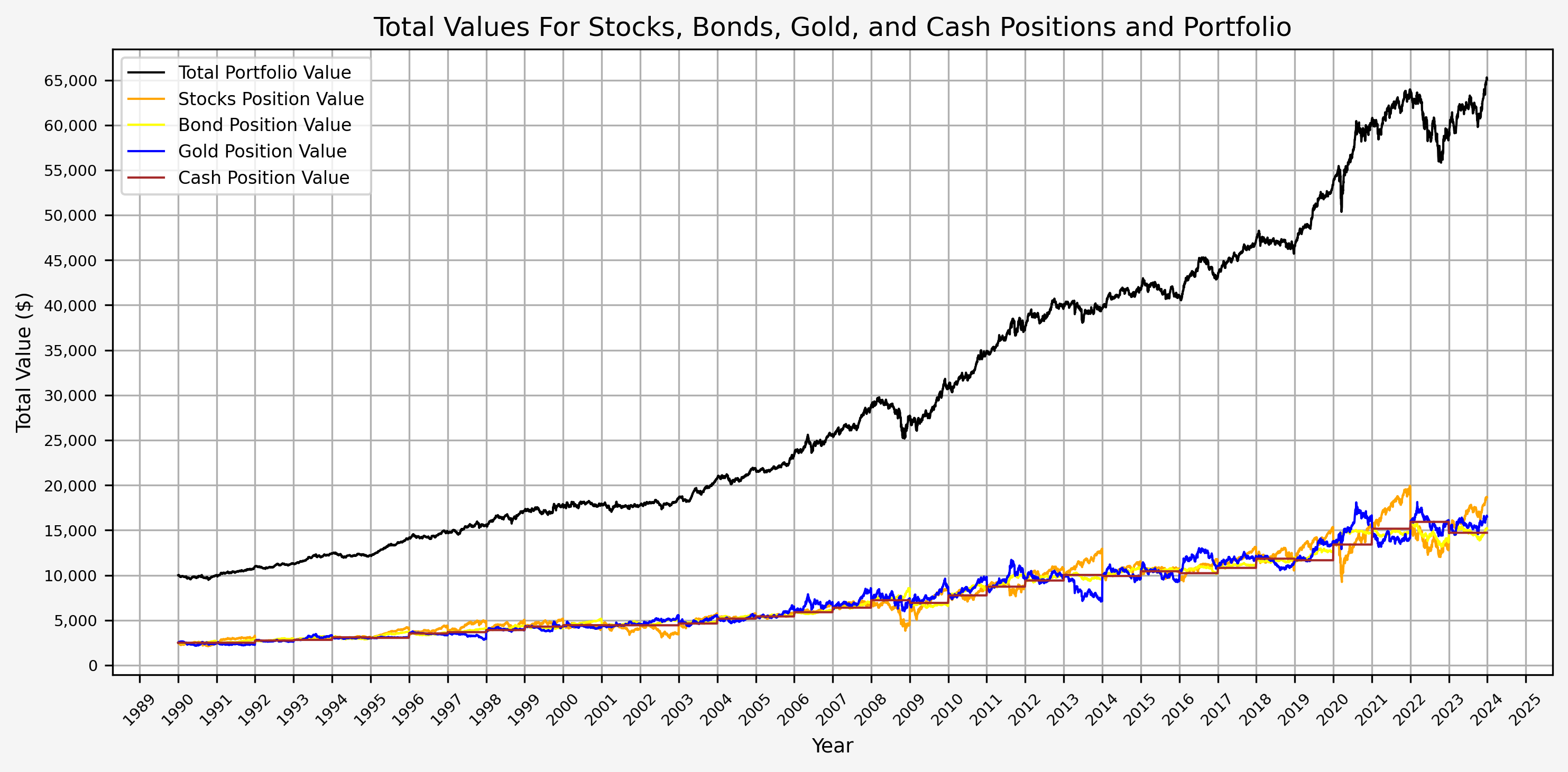
Here we can see the annual rebalancing taking effect with the values of the different asset classes. This can also be seen more clearly below.

Portfolio Drawdown

Portfolio Drawdown

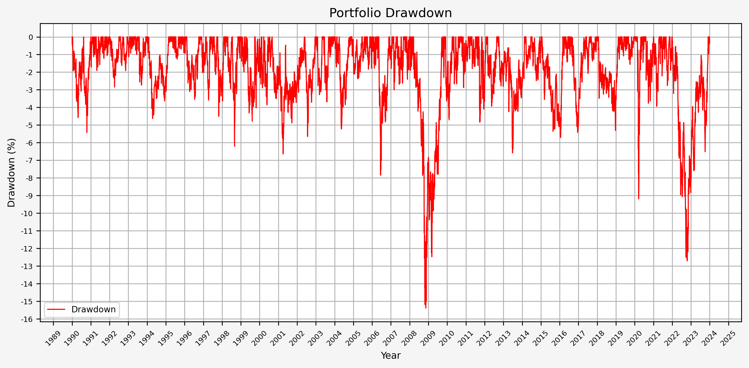
From this plot, we can see that the maximum drawdown came during the GFC; the drawdown during COVID was (interestingly) less than 10%.

Portfolio Asset Weights

Portfolio Weights

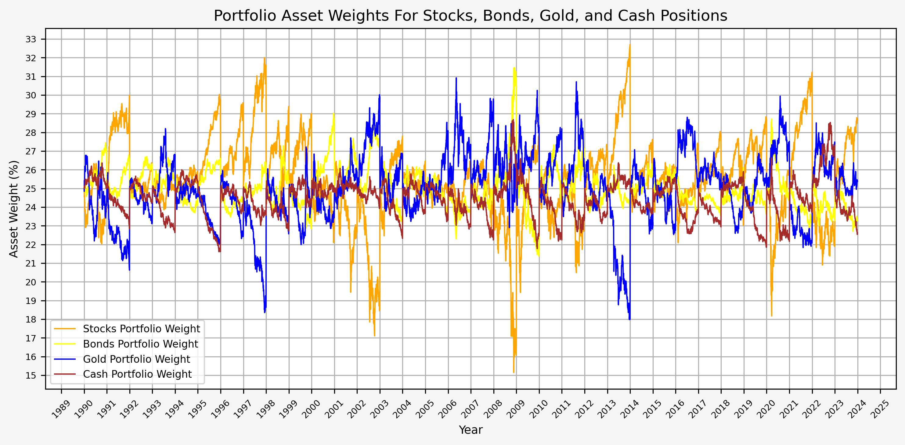
The annual rebalancing appears to work effectively by selling assets that have increased in value and buying assets that have decreased in value over the previous year. Also note that there is only one instance when the weight of an asset fell to 15%. This occured for stocks during the GFC.

Portfolio Annual Returns

Portfolio Annual Returns

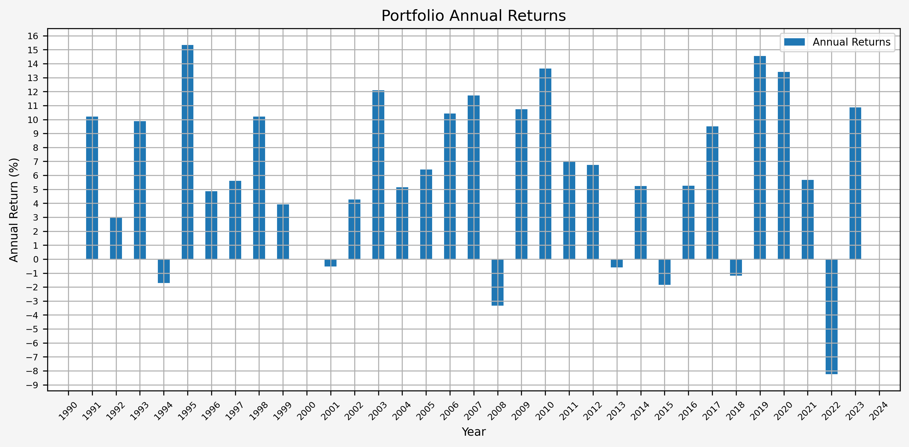
It’s interesting to see that there really aren’t any significant up or down years. Instead, it’s a steady climb without much volatility.

Summary

Overall, this is an interesting case study and Browne’s idea behind the Permanent Portfolio is certainly compelling. There might be more investigation to be done with respect to the following:

Investigate the extent to which the rebalancing date effects the portfolio performance
Vary the weights of the asset classes to see if there is a meanful change in the results
Experiment with leverage (i.e., simulating 1.2x leverage with a portfolio with weights of 30, 30, 30, 10 for stocks, bonds, gold, cash respectively.)
Use ETFs instead of Bloomberg index data, and verify the results are similar. ETF data is much more available than the Bloomberg index.

References

Fail-Safe Investing: Lifelong Financial Security in 30 Minutes, by Harry Browne

Code

The jupyter notebook with the functions and all other code is available here.
The html export of the jupyter notebook is available here.
The pdf export of the jupyter notebook is available here.